Colour is an open-source Python package providing a comprehensive number of algorithms and datasets for colour science.
It is freely available under the New BSD License terms.
Colour is an affiliated project of NumFOCUS, a 501(c)(3) nonprofit in the United States.
1 Draft Release Notes
The draft release notes from the develop branch are available at this url.
2 Sponsors
We are grateful for the support of our sponsors. If you’d like to join them, please consider becoming a sponsor on OpenCollective.
3 Features
Most of the objects are available from the colour namespace:
>>> import colour
3.1 Automatic Colour Conversion Graph - colour.graph
Starting with version 0.3.14, Colour implements an automatic colour conversion graph enabling easier colour conversions.
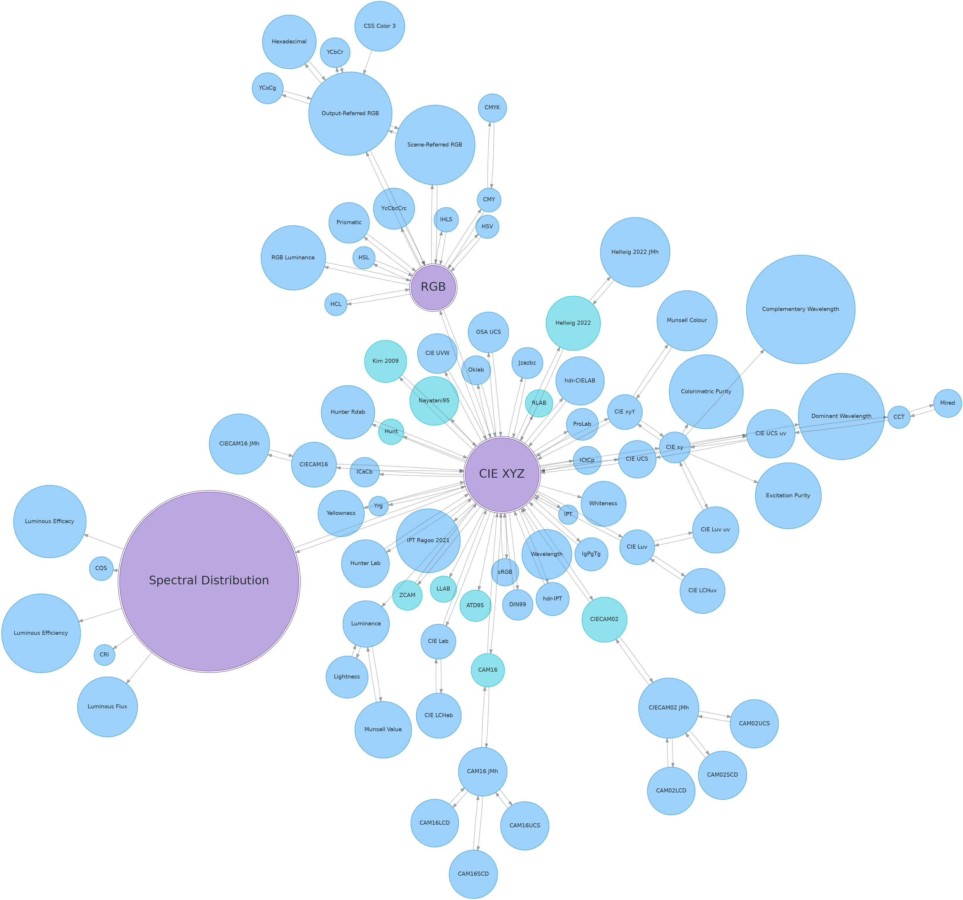
>>> sd = colour.SDS_COLOURCHECKERS['ColorChecker N Ohta']['dark skin']
>>> colour.convert(sd, 'Spectral Distribution', 'sRGB', verbose={'mode': 'Short'})
===============================================================================
* *
* [ Conversion Path ] *
* *
* "sd_to_XYZ" --> "XYZ_to_sRGB" *
* *
===============================================================================
array([ 0.45675795, 0.30986982, 0.24861924])
>>> illuminant = colour.SDS_ILLUMINANTS['FL2']
>>> colour.convert(sd, 'Spectral Distribution', 'sRGB', sd_to_XYZ={'illuminant': illuminant})
array([ 0.47924575, 0.31676968, 0.17362725])
3.2 Chromatic Adaptation - colour.adaptation
>>> XYZ = [0.20654008, 0.12197225, 0.05136952]
>>> D65 = colour.CCS_ILLUMINANTS['CIE 1931 2 Degree Standard Observer']['D65']
>>> A = colour.CCS_ILLUMINANTS['CIE 1931 2 Degree Standard Observer']['A']
>>> colour.chromatic_adaptation(
... XYZ, colour.xy_to_XYZ(D65), colour.xy_to_XYZ(A))
array([ 0.2533053 , 0.13765138, 0.01543307])
>>> sorted(colour.CHROMATIC_ADAPTATION_METHODS)
['CIE 1994', 'CMCCAT2000', 'Fairchild 1990', 'Von Kries', 'Zhai 2018']
3.3 Algebra - colour.algebra
3.3.1 Kernel Interpolation
>>> y = [5.9200, 9.3700, 10.8135, 4.5100, 69.5900, 27.8007, 86.0500]
>>> x = range(len(y))
>>> colour.KernelInterpolator(x, y)([0.25, 0.75, 5.50])
array([ 6.18062083, 8.08238488, 57.85783403])
3.3.2 Sprague (1880) Interpolation
>>> y = [5.9200, 9.3700, 10.8135, 4.5100, 69.5900, 27.8007, 86.0500]
>>> x = range(len(y))
>>> colour.SpragueInterpolator(x, y)([0.25, 0.75, 5.50])
array([ 6.72951612, 7.81406251, 43.77379185])
3.4 Colour Appearance Models - colour.appearance
>>> XYZ = [0.20654008 * 100, 0.12197225 * 100, 0.05136952 * 100]
>>> XYZ_w = [95.05, 100.00, 108.88]
>>> L_A = 318.31
>>> Y_b = 20.0
>>> colour.XYZ_to_CIECAM02(XYZ, XYZ_w, L_A, Y_b)
CAM_Specification_CIECAM02(J=34.434525727858997, C=67.365010921125943, h=22.279164147957065, s=62.81485585332716, Q=177.47124941102123, M=70.024939419291414, H=2.6896085344238898, HC=None)
>>> colour.XYZ_to_CAM16(XYZ, XYZ_w, L_A, Y_b)
CAM_Specification_CAM16(J=33.880368498111686, C=69.444353357408033, h=19.510887327451748, s=64.03612114840314, Q=176.03752758512178, M=72.18638534116765, H=399.52975599115319, HC=None)
>>> colour.XYZ_to_Kim2009(XYZ, XYZ_w, L_A)
CAM_Specification_Kim2009(J=19.879918542450902, C=55.839055250876946, h=22.013388165090046, s=112.97979354939129, Q=36.309026130161449, M=46.346415858227864, H=2.3543198369639931, HC=None)
>>> colour.XYZ_to_ZCAM(XYZ, XYZ_w, L_A, Y_b)
CAM_Specification_ZCAM(J=38.347186278956357, C=21.12138989208518, h=33.711578931095197, s=81.444585609489536, Q=76.986725284523772, M=42.403805833900506, H=0.45779200212219573, HC=None, V=43.623590687423544, K=43.20894953152817, W=34.829588380192149)
3.5 Colour Blindness - colour.blindness
>>> import numpy as np
>>> cmfs = colour.LMS_CMFS['Stockman & Sharpe 2 Degree Cone Fundamentals']
>>> colour.msds_cmfs_anomalous_trichromacy_Machado2009(cmfs, np.array([15, 0, 0]))[450]
array([ 0.08912884, 0.0870524 , 0.955393 ])
>>> primaries = colour.MSDS_DISPLAY_PRIMARIES['Apple Studio Display']
>>> d_LMS = (15, 0, 0)
>>> colour.matrix_anomalous_trichromacy_Machado2009(cmfs, primaries, d_LMS)
array([[-0.27774652, 2.65150084, -1.37375432],
[ 0.27189369, 0.20047862, 0.52762768],
[ 0.00644047, 0.25921579, 0.73434374]])
3.6 Colour Correction - colour characterisation
>>> import numpy as np
>>> RGB = [0.17224810, 0.09170660, 0.06416938]
>>> M_T = np.random.random((24, 3))
>>> M_R = M_T + (np.random.random((24, 3)) - 0.5) * 0.5
>>> colour.colour_correction(RGB, M_T, M_R)
array([ 0.1806237 , 0.07234791, 0.07848845])
>>> sorted(colour.COLOUR_CORRECTION_METHODS)
['Cheung 2004', 'Finlayson 2015', 'Vandermonde']
3.7 ACES Input Transform - colour characterisation
>>> sensitivities = colour.MSDS_CAMERA_SENSITIVITIES['Nikon 5100 (NPL)']
>>> illuminant = colour.SDS_ILLUMINANTS['D55']
>>> colour.matrix_idt(sensitivities, illuminant)
(array([[ 0.46579986, 0.13409221, 0.01935163],
[ 0.01786092, 0.77557268, -0.16775531],
[ 0.03458647, -0.16152923, 0.74270363]]), array([ 1.58214188, 1. , 1.28910346]))
3.8 Colorimetry - colour.colorimetry
3.8.1 Spectral Computations
>>> colour.sd_to_XYZ(colour.SDS_LIGHT_SOURCES['Neodimium Incandescent'])
array([ 36.94726204, 32.62076174, 13.0143849 ])
>>> sorted(colour.SPECTRAL_TO_XYZ_METHODS)
['ASTM E308', 'Integration', 'astm2015']
3.8.2 Multi-Spectral Computations
>>> msds = np.array([
... [[0.01367208, 0.09127947, 0.01524376, 0.02810712, 0.19176012, 0.04299992],
... [0.00959792, 0.25822842, 0.41388571, 0.22275120, 0.00407416, 0.37439537],
... [0.01791409, 0.29707789, 0.56295109, 0.23752193, 0.00236515, 0.58190280]],
... [[0.01492332, 0.10421912, 0.02240025, 0.03735409, 0.57663846, 0.32416266],
... [0.04180972, 0.26402685, 0.03572137, 0.00413520, 0.41808194, 0.24696727],
... [0.00628672, 0.11454948, 0.02198825, 0.39906919, 0.63640803, 0.01139849]],
... [[0.04325933, 0.26825359, 0.23732357, 0.05175860, 0.01181048, 0.08233768],
... [0.02484169, 0.12027161, 0.00541695, 0.00654612, 0.18603799, 0.36247808],
... [0.03102159, 0.16815442, 0.37186235, 0.08610666, 0.00413520, 0.78492409]],
... [[0.11682307, 0.78883040, 0.74468607, 0.83375293, 0.90571451, 0.70054168],
... [0.06321812, 0.41898224, 0.15190357, 0.24591440, 0.55301750, 0.00657664],
... [0.00305180, 0.11288624, 0.11357290, 0.12924391, 0.00195315, 0.21771573]],
... ])
>>> colour.msds_to_XYZ(msds, method='Integration',
... shape=colour.SpectralShape(400, 700, 60))
array([[[ 7.68544647, 4.09414317, 8.49324254],
[ 17.12567298, 27.77681821, 25.52573685],
[ 19.10280411, 34.45851476, 29.76319628]],
[[ 18.03375827, 8.62340812, 9.71702574],
[ 15.03110867, 6.54001068, 24.53208465],
[ 37.68269495, 26.4411103 , 10.66361816]],
[[ 8.09532373, 12.75333339, 25.79613956],
[ 7.09620297, 2.79257389, 11.15039854],
[ 8.933163 , 19.39985815, 17.14915636]],
[[ 80.00969553, 80.39810464, 76.08184429],
[ 33.27611427, 24.38947838, 39.34919287],
[ 8.89425686, 11.05185138, 10.86767594]]])
>>> sorted(colour.MSDS_TO_XYZ_METHODS)
['ASTM E308', 'Integration', 'astm2015']
3.8.3 Blackbody Spectral Radiance Computation
>>> colour.sd_blackbody(5000)
SpectralDistribution([[ 3.60000000e+02, 6.65427827e+12],
[ 3.61000000e+02, 6.70960528e+12],
[ 3.62000000e+02, 6.76482512e+12],
...
[ 7.78000000e+02, 1.06068004e+13],
[ 7.79000000e+02, 1.05903327e+13],
[ 7.80000000e+02, 1.05738520e+13]],
interpolator=SpragueInterpolator,
interpolator_args={},
extrapolator=Extrapolator,
extrapolator_args={'right': None, 'method': 'Constant', 'left': None})
3.8.4 Dominant, Complementary Wavelength & Colour Purity Computation
>>> xy = [0.54369557, 0.32107944]
>>> xy_n = [0.31270000, 0.32900000]
>>> colour.dominant_wavelength(xy, xy_n)
(array(616.0),
array([ 0.68354746, 0.31628409]),
array([ 0.68354746, 0.31628409]))
3.8.5 Lightness Computation
>>> colour.lightness(12.19722535)
41.527875844653451
>>> sorted(colour.LIGHTNESS_METHODS)
['Abebe 2017',
'CIE 1976',
'Fairchild 2010',
'Fairchild 2011',
'Glasser 1958',
'Lstar1976',
'Wyszecki 1963']
3.8.6 Luminance Computation
>>> colour.luminance(41.52787585)
12.197225353400775
>>> sorted(colour.LUMINANCE_METHODS)
['ASTM D1535',
'CIE 1976',
'Fairchild 2010',
'Fairchild 2011',
'Newhall 1943',
'astm2008',
'cie1976']
3.8.7 Whiteness Computation
>>> XYZ = [95.00000000, 100.00000000, 105.00000000]
>>> XYZ_0 = [94.80966767, 100.00000000, 107.30513595]
>>> colour.whiteness(XYZ, XYZ_0)
array([ 93.756 , -1.33000001])
>>> sorted(colour.WHITENESS_METHODS)
['ASTM E313',
'Berger 1959',
'CIE 2004',
'Ganz 1979',
'Stensby 1968',
'Taube 1960',
'cie2004']
3.8.8 Yellowness Computation
>>> XYZ = [95.00000000, 100.00000000, 105.00000000]
>>> colour.yellowness(XYZ)
4.3400000000000034
>>> sorted(colour.YELLOWNESS_METHODS)
['ASTM D1925', 'ASTM E313', 'ASTM E313 Alternative']
3.8.9 Luminous Flux, Efficiency & Efficacy Computation
>>> sd = colour.SDS_LIGHT_SOURCES['Neodimium Incandescent']
>>> colour.luminous_flux(sd)
23807.655527367202
>>> sd = colour.SDS_LIGHT_SOURCES['Neodimium Incandescent']
>>> colour.luminous_efficiency(sd)
0.19943935624521045
>>> sd = colour.SDS_LIGHT_SOURCES['Neodimium Incandescent']
>>> colour.luminous_efficacy(sd)
136.21708031547874
3.9 Contrast Sensitivity Function - colour.contrast
>>> colour.contrast_sensitivity_function(u=4, X_0=60, E=65)
358.51180789884984
>>> sorted(colour.CONTRAST_SENSITIVITY_METHODS)
['Barten 1999']
3.10 Colour Difference - colour.difference
>>> Lab_1 = [100.00000000, 21.57210357, 272.22819350]
>>> Lab_2 = [100.00000000, 426.67945353, 72.39590835]
>>> colour.delta_E(Lab_1, Lab_2)
94.035649026659485
>>> sorted(colour.DELTA_E_METHODS)
['CAM02-LCD',
'CAM02-SCD',
'CAM02-UCS',
'CAM16-LCD',
'CAM16-SCD',
'CAM16-UCS',
'CIE 1976',
'CIE 1994',
'CIE 2000',
'CMC',
'DIN99',
'cie1976',
'cie1994',
'cie2000']
3.11 IO - colour.io
3.11.1 Images
>>> RGB = colour.read_image('Ishihara_Colour_Blindness_Test_Plate_3.png')
>>> RGB.shape
(276, 281, 3)
3.11.2 Look Up Table (LUT) Data
>>> LUT = colour.read_LUT('ACES_Proxy_10_to_ACES.cube')
>>> print(LUT)
LUT3x1D - ACES Proxy 10 to ACES
-------------------------------
Dimensions : 2
Domain : [[0 0 0]
[1 1 1]]
Size : (32, 3)
>>> RGB = [0.17224810, 0.09170660, 0.06416938]
>>> LUT.apply(RGB)
array([ 0.00575674, 0.00181493, 0.00121419])
3.12 Colour Models - colour.models
3.12.1 CIE xyY Colourspace
>>> colour.XYZ_to_xyY([0.20654008, 0.12197225, 0.05136952])
array([ 0.54369557, 0.32107944, 0.12197225])
3.12.2 CIE L*a*b* Colourspace
>>> colour.XYZ_to_Lab([0.20654008, 0.12197225, 0.05136952])
array([ 41.52787529, 52.63858304, 26.92317922])
3.12.3 CIE L*u*v* Colourspace
>>> colour.XYZ_to_Luv([0.20654008, 0.12197225, 0.05136952])
array([ 41.52787529, 96.83626054, 17.75210149])
3.12.4 CIE 1960 UCS Colourspace
>>> colour.XYZ_to_UCS([0.20654008, 0.12197225, 0.05136952])
array([ 0.13769339, 0.12197225, 0.1053731 ])
3.12.5 CIE 1964 U*V*W* Colourspace
>>> XYZ = [0.20654008 * 100, 0.12197225 * 100, 0.05136952 * 100]
>>> colour.XYZ_to_UVW(XYZ)
array([ 94.55035725, 11.55536523, 40.54757405])
3.12.6 Hunter L,a,b Colour Scale
>>> XYZ = [0.20654008 * 100, 0.12197225 * 100, 0.05136952 * 100]
>>> colour.XYZ_to_Hunter_Lab(XYZ)
array([ 34.92452577, 47.06189858, 14.38615107])
3.12.7 Hunter Rd,a,b Colour Scale
>>> XYZ = [0.20654008 * 100, 0.12197225 * 100, 0.05136952 * 100]
>>> colour.XYZ_to_Hunter_Rdab(XYZ)
array([ 12.197225 , 57.12537874, 17.46241341])
3.12.8 CAM02-LCD, CAM02-SCD, and CAM02-UCS Colourspaces - Luo, Cui and Li (2006)
>>> XYZ = [0.20654008 * 100, 0.12197225 * 100, 0.05136952 * 100]
>>> XYZ_w = [95.05, 100.00, 108.88]
>>> L_A = 318.31
>>> Y_b = 20.0
>>> surround = colour.VIEWING_CONDITIONS_CIECAM02['Average']
>>> specification = colour.XYZ_to_CIECAM02(
XYZ, XYZ_w, L_A, Y_b, surround)
>>> JMh = (specification.J, specification.M, specification.h)
>>> colour.JMh_CIECAM02_to_CAM02UCS(JMh)
array([ 47.16899898, 38.72623785, 15.8663383 ])
>>> XYZ = [0.20654008, 0.12197225, 0.05136952]
>>> XYZ_w = [95.05 / 100, 100.00 / 100, 108.88 / 100]
>>> colour.XYZ_to_CAM02UCS(XYZ, XYZ_w=XYZ_w, L_A=L_A, Y_b=Y_b)
array([ 47.16899898, 38.72623785, 15.8663383 ])
3.12.9 CAM16-LCD, CAM16-SCD, and CAM16-UCS Colourspaces - Li et al. (2017)
>>> XYZ = [0.20654008 * 100, 0.12197225 * 100, 0.05136952 * 100]
>>> XYZ_w = [95.05, 100.00, 108.88]
>>> L_A = 318.31
>>> Y_b = 20.0
>>> surround = colour.VIEWING_CONDITIONS_CAM16['Average']
>>> specification = colour.XYZ_to_CAM16(
XYZ, XYZ_w, L_A, Y_b, surround)
>>> JMh = (specification.J, specification.M, specification.h)
>>> colour.JMh_CAM16_to_CAM16UCS(JMh)
array([ 46.55542238, 40.22460974, 14.25288392]
>>> XYZ = [0.20654008, 0.12197225, 0.05136952]
>>> XYZ_w = [95.05 / 100, 100.00 / 100, 108.88 / 100]
>>> colour.XYZ_to_CAM16UCS(XYZ, XYZ_w=XYZ_w, L_A=L_A, Y_b=Y_b)
array([ 46.55542238, 40.22460974, 14.25288392])
3.12.10 ICaCb Colourspace
>>> XYZ_to_ICaCb(np.array([0.20654008, 0.12197225, 0.05136952]))
array([ 0.06875297, 0.05753352, 0.02081548])
3.12.11 IgPgTg Colourspace
>>> colour.XYZ_to_IgPgTg([0.20654008, 0.12197225, 0.05136952])
array([ 0.42421258, 0.18632491, 0.10689223])
3.12.12 IPT Colourspace
>>> colour.XYZ_to_IPT([0.20654008, 0.12197225, 0.05136952])
array([ 0.38426191, 0.38487306, 0.18886838])
3.12.13 DIN99 Colourspace
>>> Lab = [41.52787529, 52.63858304, 26.92317922]
>>> colour.Lab_to_DIN99(Lab)
array([ 53.22821988, 28.41634656, 3.89839552])
3.12.14 hdr-CIELAB Colourspace
>>> colour.XYZ_to_hdr_CIELab([0.20654008, 0.12197225, 0.05136952])
array([ 51.87002062, 60.4763385 , 32.14551912])
3.12.15 hdr-IPT Colourspace
>>> colour.XYZ_to_hdr_IPT([0.20654008, 0.12197225, 0.05136952])
array([ 25.18261761, -22.62111297, 3.18511729])
3.12.16 Oklab Colourspace
>>> colour.XYZ_to_Oklab([0.20654008, 0.12197225, 0.05136952])
array([ 0.51634019, 0.154695 , 0.06289579])
3.12.17 OSA UCS Colourspace
>>> XYZ = [0.20654008 * 100, 0.12197225 * 100, 0.05136952 * 100]
>>> colour.XYZ_to_OSA_UCS(XYZ)
array([-3.0049979 , 2.99713697, -9.66784231])
3.12.18 ProLab Colourspace
>>> colour.XYZ_to_ProLab([0.51634019, 0.15469500, 0.06289579])
array([1.24610688, 2.39525236, 0.41902126])
3.12.19 Jzazbz Colourspace
>>> colour.XYZ_to_Jzazbz([0.20654008, 0.12197225, 0.05136952])
array([ 0.00535048, 0.00924302, 0.00526007])
3.12.20 Y’CbCr Colour Encoding
>>> colour.RGB_to_YCbCr([1.0, 1.0, 1.0])
array([ 0.92156863, 0.50196078, 0.50196078])
3.12.21 YCoCg Colour Encoding
>>> colour.RGB_to_YCoCg([0.75, 0.75, 0.0])
array([ 0.5625, 0.375 , 0.1875])
3.12.22 ICtCp Colour Encoding
>>> colour.RGB_to_ICtCp([0.45620519, 0.03081071, 0.04091952])
array([ 0.07351364, 0.00475253, 0.09351596])
3.12.23 HSV Colourspace
>>> colour.RGB_to_HSV([0.45620519, 0.03081071, 0.04091952])
array([ 0.99603944, 0.93246304, 0.45620519])
3.12.24 IHLS Colourspace
>>> colour.RGB_to_IHLS([0.45620519, 0.03081071, 0.04091952])
array([ 6.26236117, 0.12197943, 0.42539448])
3.12.25 Prismatic Colourspace
>>> colour.RGB_to_Prismatic([0.25, 0.50, 0.75])
array([ 0.75 , 0.16666667, 0.33333333, 0.5 ])
3.12.26 RGB Colourspace and Transformations
>>> XYZ = [0.21638819, 0.12570000, 0.03847493]
>>> illuminant_XYZ = [0.34570, 0.35850]
>>> illuminant_RGB = [0.31270, 0.32900]
>>> chromatic_adaptation_transform = 'Bradford'
>>> matrix_XYZ_to_RGB = [
[3.24062548, -1.53720797, -0.49862860],
[-0.96893071, 1.87575606, 0.04151752],
[0.05571012, -0.20402105, 1.05699594]]
>>> colour.XYZ_to_RGB(
XYZ,
illuminant_XYZ,
illuminant_RGB,
matrix_XYZ_to_RGB,
chromatic_adaptation_transform)
array([ 0.45595571, 0.03039702, 0.04087245])
3.12.27 RGB Colourspace Derivation
>>> p = [0.73470, 0.26530, 0.00000, 1.00000, 0.00010, -0.07700]
>>> w = [0.32168, 0.33767]
>>> colour.normalised_primary_matrix(p, w)
array([[ 9.52552396e-01, 0.00000000e+00, 9.36786317e-05],
[ 3.43966450e-01, 7.28166097e-01, -7.21325464e-02],
[ 0.00000000e+00, 0.00000000e+00, 1.00882518e+00]])
3.12.28 RGB Colourspaces
>>> sorted(colour.RGB_COLOURSPACES)
['ACES2065-1',
'ACEScc',
'ACEScct',
'ACEScg',
'ACESproxy',
'ALEXA Wide Gamut',
'Adobe RGB (1998)',
'Adobe Wide Gamut RGB',
'Apple RGB',
'Best RGB',
'Beta RGB',
'Blackmagic Wide Gamut'
'CIE RGB',
'Cinema Gamut',
'ColorMatch RGB',
'DaVinci Wide Gamut',
'DCDM XYZ',
'DCI-P3',
'DCI-P3+',
'DJI D-Gamut',
'DRAGONcolor',
'DRAGONcolor2',
'Display P3',
'Don RGB 4',
'ECI RGB v2',
'ERIMM RGB',
'Ekta Space PS 5',
'F-Gamut',
'FilmLight E-Gamut',
'ITU-R BT.2020',
'ITU-R BT.470 - 525',
'ITU-R BT.470 - 625',
'ITU-R BT.709',
'Max RGB',
'NTSC (1953)',
'NTSC (1987)',
'P3-D65',
'Pal/Secam',
'ProPhoto RGB',
'Protune Native',
'REDWideGamutRGB',
'REDcolor',
'REDcolor2',
'REDcolor3',
'REDcolor4',
'RIMM RGB',
'ROMM RGB',
'Russell RGB',
'S-Gamut',
'S-Gamut3',
'S-Gamut3.Cine',
'SMPTE 240M',
'SMPTE C',
'Sharp RGB',
'V-Gamut',
'Venice S-Gamut3',
'Venice S-Gamut3.Cine',
'Xtreme RGB',
'aces',
'adobe1998',
'prophoto',
3.12.29 OETFs
>>> sorted(colour.OETFS)
['ARIB STD-B67',
'Blackmagic Film Generation 5',
'DaVinci Intermediate',
'ITU-R BT.2100 HLG',
'ITU-R BT.2100 PQ',
'ITU-R BT.601',
'ITU-R BT.709',
'SMPTE 240M']
3.12.30 EOTFs
>>> sorted(colour.EOTFS)
['DCDM',
'DICOM GSDF',
'ITU-R BT.1886',
'ITU-R BT.2020',
'ITU-R BT.2100 HLG',
'ITU-R BT.2100 PQ',
'SMPTE 240M',
'ST 2084',
'sRGB']
3.12.31 OOTFs
>>> sorted(colour.OOTFS)
['ITU-R BT.2100 HLG', 'ITU-R BT.2100 PQ']
3.12.32 Log Encoding / Decoding
>>> sorted(colour.LOG_ENCODINGS)
['ACEScc',
'ACEScct',
'ACESproxy',
'ALEXA Log C',
'Canon Log',
'Canon Log 2',
'Canon Log 3',
'Cineon',
'D-Log',
'ERIMM RGB',
'F-Log',
'Filmic Pro 6',
'Log2',
'Log3G10',
'Log3G12',
'N-Log',
'PLog',
'Panalog',
'Protune',
'REDLog',
'REDLogFilm',
'S-Log',
'S-Log2',
'S-Log3',
'T-Log',
'V-Log',
'ViperLog']
3.12.33 CCTFs Encoding / Decoding
>>> sorted(colour.CCTF_ENCODINGS)
['ACEScc',
'ACEScct',
'ACESproxy',
'ALEXA Log C',
'ARIB STD-B67',
'Canon Log',
'Canon Log 2',
'Canon Log 3',
'Cineon',
'D-Log',
'DCDM',
'DICOM GSDF',
'ERIMM RGB',
'F-Log',
'Filmic Pro 6',
'Gamma 2.2',
'Gamma 2.4',
'Gamma 2.6',
'ITU-R BT.1886',
'ITU-R BT.2020',
'ITU-R BT.2100 HLG',
'ITU-R BT.2100 PQ',
'ITU-R BT.601',
'ITU-R BT.709',
'Log2',
'Log3G10',
'Log3G12',
'PLog',
'Panalog',
'ProPhoto RGB',
'Protune',
'REDLog',
'REDLogFilm',
'RIMM RGB',
'ROMM RGB',
'S-Log',
'S-Log2',
'S-Log3',
'SMPTE 240M',
'ST 2084',
'T-Log',
'V-Log',
'ViperLog',
'sRGB']
3.13 Colour Notation Systems - colour.notation
3.13.1 Munsell Value
>>> colour.munsell_value(12.23634268)
4.0824437076525664
>>> sorted(colour.MUNSELL_VALUE_METHODS)
['ASTM D1535',
'Ladd 1955',
'McCamy 1987',
'Moon 1943',
'Munsell 1933',
'Priest 1920',
'Saunderson 1944',
'astm2008']
3.13.2 Munsell Colour
>>> colour.xyY_to_munsell_colour([0.38736945, 0.35751656, 0.59362000])
'4.2YR 8.1/5.3'
>>> colour.munsell_colour_to_xyY('4.2YR 8.1/5.3')
array([ 0.38736945, 0.35751656, 0.59362 ])
3.14 Optical Phenomena - colour.phenomena
>>> colour.rayleigh_scattering_sd()
SpectralDistribution([[ 3.60000000e+02, 5.99101337e-01],
[ 3.61000000e+02, 5.92170690e-01],
[ 3.62000000e+02, 5.85341006e-01],
...
[ 7.78000000e+02, 2.55208377e-02],
[ 7.79000000e+02, 2.53887969e-02],
[ 7.80000000e+02, 2.52576106e-02]],
interpolator=SpragueInterpolator,
interpolator_args={},
extrapolator=Extrapolator,
extrapolator_args={'right': None, 'method': 'Constant', 'left': None})
3.15 Light Quality - colour.quality
3.15.1 Colour Fidelity Index
>>> colour.colour_fidelity_index(colour.SDS_ILLUMINANTS['FL2'])
70.120825477833037
>>> sorted(colour.COLOUR_FIDELITY_INDEX_METHODS)
['ANSI/IES TM-30-18', 'CIE 2017']
3.15.2 Colour Rendering Index
>>> colour.colour_quality_scale(colour.SDS_ILLUMINANTS['FL2'])
64.111703163816699
>>> sorted(colour.COLOUR_QUALITY_SCALE_METHODS)
['NIST CQS 7.4', 'NIST CQS 9.0']
3.15.3 Colour Quality Scale
>>> colour.colour_rendering_index(colour.SDS_ILLUMINANTS['FL2'])
64.233724121664807
3.15.4 Academy Spectral Similarity Index (SSI)
>>> colour.spectral_similarity_index(colour.SDS_ILLUMINANTS['C'], colour.SDS_ILLUMINANTS['D65'])
94.0
3.16 Spectral Up-Sampling & Reflectance Recovery - colour.recovery
>>> colour.XYZ_to_sd([0.20654008, 0.12197225, 0.05136952])
SpectralDistribution([[ 3.60000000e+02, 8.37868873e-02],
[ 3.65000000e+02, 8.39337988e-02],
...
[ 7.70000000e+02, 4.46793405e-01],
[ 7.75000000e+02, 4.46872853e-01],
[ 7.80000000e+02, 4.46914431e-01]],
interpolator=SpragueInterpolator,
interpolator_kwargs={},
extrapolator=Extrapolator,
extrapolator_kwargs={'method': 'Constant', 'left': None, 'right': None})
>>> sorted(colour.REFLECTANCE_RECOVERY_METHODS)
['Jakob 2019', 'Mallett 2019', 'Meng 2015', 'Otsu 2018', 'Smits 1999']
3.18 Colour Volume - colour.volume
>>> colour.RGB_colourspace_volume_MonteCarlo(colour.RGB_COLOURSPACE_RGB['sRGB'])
821958.30000000005
3.19 Geometry Primitives Generation - colour.geometry
>>> colour.primitive('Grid')
(array([ ([-0.5, 0.5, 0. ], [ 0., 1.], [ 0., 0., 1.], [ 0., 1., 0., 1.]),
([ 0.5, 0.5, 0. ], [ 1., 1.], [ 0., 0., 1.], [ 1., 1., 0., 1.]),
([-0.5, -0.5, 0. ], [ 0., 0.], [ 0., 0., 1.], [ 0., 0., 0., 1.]),
([ 0.5, -0.5, 0. ], [ 1., 0.], [ 0., 0., 1.], [ 1., 0., 0., 1.])],
dtype=[('position', '<f4', (3,)), ('uv', '<f4', (2,)), ('normal', '<f4', (3,)), ('colour', '<f4', (4,))]), array([[0, 2, 1],
[2, 3, 1]], dtype=uint32), array([[0, 2],
[2, 3],
[3, 1],
[1, 0]], dtype=uint32))
>>> sorted(colour.PRIMITIVE_METHODS)
['Cube', 'Grid']
>>> colour.primitive_vertices('Quad MPL')
array([[ 0., 0., 0.],
[ 1., 0., 0.],
[ 1., 1., 0.],
[ 0., 1., 0.]])
>>> sorted(colour.PRIMITIVE_VERTICES_METHODS)
['Cube MPL', 'Grid MPL', 'Quad MPL', 'Sphere']
3.20 Plotting - colour.plotting
Most of the objects are available from the colour.plotting namespace:
>>> from colour.plotting import *
>>> colour_style()
3.20.1 Visible Spectrum
>>> plot_visible_spectrum('CIE 1931 2 Degree Standard Observer')

3.20.2 Spectral Distribution
>>> plot_single_illuminant_sd('FL1')

3.20.3 Blackbody
>>> blackbody_sds = [
... colour.sd_blackbody(i, colour.SpectralShape(0, 10000, 10))
... for i in range(1000, 15000, 1000)
... ]
>>> plot_multi_sds(
... blackbody_sds,
... y_label='W / (sr m$^2$) / m',
... plot_kwargs={
... 'use_sd_colours': True,
... 'normalise_sd_colours': True,
... },
... legend_location='upper right',
... bounding_box=(0, 1250, 0, 2.5e6))

3.20.4 Colour Matching Functions
>>> plot_single_cmfs(
... 'Stockman & Sharpe 2 Degree Cone Fundamentals',
... y_label='Sensitivity',
... bounding_box=(390, 870, 0, 1.1))

3.20.5 Luminous Efficiency
>>> sd_mesopic_luminous_efficiency_function = (
... colour.sd_mesopic_luminous_efficiency_function(0.2))
>>> plot_multi_sds(
... (sd_mesopic_luminous_efficiency_function,
... colour.PHOTOPIC_LEFS['CIE 1924 Photopic Standard Observer'],
... colour.SCOTOPIC_LEFS['CIE 1951 Scotopic Standard Observer']),
... y_label='Luminous Efficiency',
... legend_location='upper right',
... y_tighten=True,
... margins=(0, 0, 0, 0.1))

3.20.6 Colour Checker
>>> from colour.characterisation.dataset.colour_checkers.sds import (
... COLOURCHECKER_INDEXES_TO_NAMES_MAPPING)
>>> plot_multi_sds(
... [
... colour.SDS_COLOURCHECKERS['BabelColor Average'][value]
... for key, value in sorted(
... COLOURCHECKER_INDEXES_TO_NAMES_MAPPING.items())
... ],
... plot_kwargs={
... use_sd_colours=True,
... },
... title=('BabelColor Average - '
... 'Spectral Distributions'))

>>> plot_single_colour_checker(
... 'ColorChecker 2005', text_kwargs={'visible': False})

3.20.7 Chromaticities Prediction
>>> plot_corresponding_chromaticities_prediction(
... 2, 'Von Kries', 'Bianco 2010')

3.20.8 Chromaticities
>>> import numpy as np
>>> RGB = np.random.random((32, 32, 3))
>>> plot_RGB_chromaticities_in_chromaticity_diagram_CIE1931(
... RGB, 'ITU-R BT.709',
... colourspaces=['ACEScg', 'S-Gamut'], show_pointer_gamut=True)

3.20.9 Colour Rendering Index
>>> plot_single_sd_colour_rendering_index_bars(
... colour.SDS_ILLUMINANTS['FL2'])

3.20.10 ANSI/IES TM-30-18 Colour Rendition Report
>>> plot_single_sd_colour_rendition_report(
... colour.SDS_ILLUMINANTS['FL2'])

3.20.11 Gamut Section
>>> plot_visible_spectrum_section(section_colours='RGB', section_opacity=0.15)

>>> plot_RGB_colourspace_section('sRGB', section_colours='RGB', section_opacity=0.15)

3.20.12 Colour Temperature
>>> plot_planckian_locus_in_chromaticity_diagram_CIE1960UCS(['A', 'B', 'C'])

4 User Guide
User Guide
The user guide provides an overview of Colour and explains important concepts and features, details can be found in the API Reference.
Tutorial
Note
An interactive version of the tutorial is available via Google Colab.
Colour spreads over various domains of Colour Science, from colour models to optical phenomena, this tutorial does not give a complete overview of the API but is a good introduction to the main concepts.
Note
A directory with examples is available at this path in Colour installation: colour/examples. It can also be explored directly on Github.
from colour.plotting import *
colour_style()
plot_visible_spectrum()

Overview
Colour is organised around various sub-packages:
adaptation: Chromatic adaptation models and transformations.
algebra: Algebra utilities.
appearance: Colour appearance models.
biochemistry: Biochemistry computations.
blindness: Colour vision deficiency models.
characterisation: Colour correction, camera and display characterisation.
colorimetry: Core objects for colour computations.
constants: CIE and CODATA constants.
continuous: Base objects for continuous data representation.
contrast: Objects for contrast sensitivity computation.
corresponding: Corresponding colour chromaticities computations.
difference: Colour difference computations.
geometry: Geometry primitives generation.
graph: Graph for automatic colour conversions.
hints: Type hints for annotations.
io: Input / output objects for reading and writing data.
models: Colour models.
notation: Colour notation systems.
phenomena: Computation of various optical phenomena.
plotting: Diagrams, figures, etc…
quality: Colour quality computation.
recovery: Reflectance recovery.
temperature: Colour temperature and correlated colour temperature computation.
utilities: Various utilities and data structures.
volume: Colourspace volumes computation and optimal colour stimuli.
Most of the public API is available from the root colour namespace:
import colour
print(colour.__all__[:5] + ['...'])
['domain_range_scale', 'get_domain_range_scale', 'set_domain_range_scale', 'CHROMATIC_ADAPTATION_METHODS', 'CHROMATIC_ADAPTATION_TRANSFORMS', '...']
The various sub-packages also expose their public API:
from pprint import pprint
for sub_package in ('adaptation', 'algebra', 'appearance', 'biochemistry',
'blindness', 'characterisation', 'colorimetry',
'constants', 'continuous', 'contrast', 'corresponding',
'difference', 'geometry', 'graph', 'hints', 'io', 'models',
'notation', 'phenomena', 'plotting', 'quality',
'recovery', 'temperature', 'utilities', 'volume'):
print(sub_package.title())
pprint(getattr(colour, sub_package).__all__[:5] + ['...'])
print('\n')
Adaptation
['CHROMATIC_ADAPTATION_TRANSFORMS',
'CAT_BIANCO2010',
'CAT_BRADFORD',
'CAT_CAT02',
'CAT_CAT02_BRILL2008',
'...']
Algebra
['cartesian_to_spherical',
'spherical_to_cartesian',
'cartesian_to_polar',
'polar_to_cartesian',
'cartesian_to_cylindrical',
'...']
Appearance
['InductionFactors_Hunt',
'VIEWING_CONDITIONS_HUNT',
'CAM_Specification_Hunt',
'XYZ_to_Hunt',
'CAM_Specification_ATD95',
'...']
Biochemistry
['REACTION_RATE_MICHAELISMENTEN_METHODS',
'reaction_rate_MichaelisMenten',
'SUBSTRATE_CONCENTRATION_MICHAELISMENTEN_METHODS',
'substrate_concentration_MichaelisMenten',
'reaction_rate_MichaelisMenten_Michaelis1913',
'...']
Blindness
['CVD_MATRICES_MACHADO2010',
'msds_cmfs_anomalous_trichromacy_Machado2009',
'matrix_anomalous_trichromacy_Machado2009',
'matrix_cvd_Machado2009',
'...']
Characterisation
['RGB_CameraSensitivities',
'RGB_DisplayPrimaries',
'MSDS_ACES_RICD',
'MSDS_CAMERA_SENSITIVITIES',
'CCS_COLOURCHECKERS',
'...']
Colorimetry
['SpectralShape',
'SPECTRAL_SHAPE_DEFAULT',
'SpectralDistribution',
'MultiSpectralDistributions',
'reshape_sd',
'...']
Constants
['CONSTANT_K_M',
'CONSTANT_KP_M',
'CONSTANT_AVOGADRO',
'CONSTANT_BOLTZMANN',
'CONSTANT_LIGHT_SPEED',
'...']
Continuous
['AbstractContinuousFunction', 'Signal', 'MultiSignals', '...']
Contrast
['optical_MTF_Barten1999',
'pupil_diameter_Barten1999',
'sigma_Barten1999',
'retinal_illuminance_Barten1999',
'maximum_angular_size_Barten1999',
'...']
Corresponding
['BRENEMAN_EXPERIMENTS',
'BRENEMAN_EXPERIMENT_PRIMARIES_CHROMATICITIES',
'CorrespondingColourDataset',
'CorrespondingChromaticitiesPrediction',
'corresponding_chromaticities_prediction_CIE1994',
'...']
Difference
['delta_E_CAM02LCD',
'delta_E_CAM02SCD',
'delta_E_CAM02UCS',
'delta_E_CAM16LCD',
'delta_E_CAM16SCD',
'...']
Geometry
['PLANE_TO_AXIS_MAPPING',
'primitive_grid',
'primitive_cube',
'hull_section',
'PRIMITIVE_METHODS',
'...']
Graph
['CONVERSION_GRAPH',
'CONVERSION_GRAPH_NODE_LABELS',
'describe_conversion_path',
'convert',
'...']
Hints
['Any', 'Callable', 'Dict', 'Generator', 'Iterable', '...']
Io
['LUT1D',
'LUT3x1D',
'LUT3D',
'LUT_to_LUT',
'AbstractLUTSequenceOperator',
'...']
Models
['Jab_to_JCh',
'JCh_to_Jab',
'COLOURSPACE_MODELS',
'COLOURSPACE_MODELS_AXIS_LABELS',
'COLOURSPACE_MODELS_DOMAIN_RANGE_SCALE_1_TO_REFERENCE',
'...']
Notation
['MUNSELL_COLOURS_ALL',
'MUNSELL_COLOURS_1929',
'MUNSELL_COLOURS_REAL',
'MUNSELL_COLOURS',
'munsell_value',
'...']
Phenomena
['scattering_cross_section',
'rayleigh_optical_depth',
'rayleigh_scattering',
'sd_rayleigh_scattering',
'...']
Plotting
['SD_ASTMG173_ETR',
'SD_ASTMG173_GLOBAL_TILT',
'SD_ASTMG173_DIRECT_CIRCUMSOLAR',
'CONSTANTS_COLOUR_STYLE',
'CONSTANTS_ARROW_STYLE',
'...']
Quality
['SDS_TCS',
'SDS_VS',
'ColourRendering_Specification_CIE2017',
'colour_fidelity_index_CIE2017',
'ColourQuality_Specification_ANSIIESTM3018',
'...']
Recovery
['SPECTRAL_SHAPE_sRGB_MALLETT2019',
'MSDS_BASIS_FUNCTIONS_sRGB_MALLETT2019',
'SPECTRAL_SHAPE_OTSU2018',
'BASIS_FUNCTIONS_OTSU2018',
'CLUSTER_MEANS_OTSU2018',
'...']
Temperature
['xy_to_CCT_CIE_D',
'CCT_to_xy_CIE_D',
'xy_to_CCT_Hernandez1999',
'CCT_to_xy_Hernandez1999',
'xy_to_CCT_Kang2002',
'...']
Utilities
['Lookup',
'Structure',
'CaseInsensitiveMapping',
'LazyCaseInsensitiveMapping',
'Node',
'...']
Volume
['OPTIMAL_COLOUR_STIMULI_ILLUMINANTS',
'is_within_macadam_limits',
'is_within_mesh_volume',
'is_within_pointer_gamut',
'generate_pulse_waves',
'...']
The codebase is documented and most docstrings have usage examples:
print(colour.temperature.CCT_to_uv_Ohno2013.__doc__)
Return the *CIE UCS* colourspace *uv* chromaticity coordinates from given
correlated colour temperature :math:`T_{cp}`, :math:`\Delta_{uv}` and
colour matching functions using *Ohno (2013)* method.
Parameters
----------
CCT_D_uv
Correlated colour temperature :math:`T_{cp}`, :math:`\Delta_{uv}`.
cmfs
Standard observer colour matching functions, default to the
*CIE 1931 2 Degree Standard Observer*.
Returns
-------
:class:`numpy.ndarray`
*CIE UCS* colourspace *uv* chromaticity coordinates.
References
----------
:cite:`Ohno2014a`
Examples
--------
>>> from pprint import pprint
>>> from colour import MSDS_CMFS, SPECTRAL_SHAPE_DEFAULT
>>> cmfs = (
... MSDS_CMFS['CIE 1931 2 Degree Standard Observer'].
... copy().align(SPECTRAL_SHAPE_DEFAULT)
... )
>>> CCT_D_uv = np.array([6507.4342201047066, 0.003223690901513])
>>> CCT_to_uv_Ohno2013(CCT_D_uv, cmfs) # doctest: +ELLIPSIS
array([ 0.1977999..., 0.3122004...])
At the core of Colour is the colour.colorimetry sub-package, it defines
the objects needed for spectral computations and many others:
pprint(colour.colorimetry.__all__)
['SpectralShape',
'SPECTRAL_SHAPE_DEFAULT',
'SpectralDistribution',
'MultiSpectralDistributions',
'reshape_sd',
'reshape_msds',
'sds_and_msds_to_sds',
'sds_and_msds_to_msds',
'sd_blackbody',
'blackbody_spectral_radiance',
'planck_law',
'LMS_ConeFundamentals',
'RGB_ColourMatchingFunctions',
'XYZ_ColourMatchingFunctions',
'CCS_ILLUMINANTS',
'MSDS_CMFS',
'MSDS_CMFS_LMS',
'MSDS_CMFS_RGB',
'MSDS_CMFS_STANDARD_OBSERVER',
'SDS_BASIS_FUNCTIONS_CIE_ILLUMINANT_D_SERIES',
'SDS_ILLUMINANTS',
'SDS_LEFS',
'SDS_LEFS_PHOTOPIC',
'SDS_LEFS_SCOTOPIC',
'TVS_ILLUMINANTS',
'TVS_ILLUMINANTS_HUNTERLAB',
'CCS_LIGHT_SOURCES',
'SDS_LIGHT_SOURCES',
'sd_constant',
'sd_zeros',
'sd_ones',
'msds_constant',
'msds_zeros',
'msds_ones',
'SD_GAUSSIAN_METHODS',
'sd_gaussian',
'sd_gaussian_normal',
'sd_gaussian_fwhm',
'SD_SINGLE_LED_METHODS',
'sd_single_led',
'sd_single_led_Ohno2005',
'SD_MULTI_LEDS_METHODS',
'sd_multi_leds',
'sd_multi_leds_Ohno2005',
'SD_TO_XYZ_METHODS',
'MSDS_TO_XYZ_METHODS',
'sd_to_XYZ',
'msds_to_XYZ',
'SPECTRAL_SHAPE_ASTME308',
'handle_spectral_arguments',
'lagrange_coefficients_ASTME2022',
'tristimulus_weighting_factors_ASTME2022',
'adjust_tristimulus_weighting_factors_ASTME308',
'sd_to_XYZ_integration',
'sd_to_XYZ_tristimulus_weighting_factors_ASTME308',
'sd_to_XYZ_ASTME308',
'msds_to_XYZ_integration',
'msds_to_XYZ_ASTME308',
'wavelength_to_XYZ',
'spectral_uniformity',
'BANDPASS_CORRECTION_METHODS',
'bandpass_correction',
'bandpass_correction_Stearns1988',
'sd_CIE_standard_illuminant_A',
'sd_CIE_illuminant_D_series',
'daylight_locus_function',
'sd_mesopic_luminous_efficiency_function',
'mesopic_weighting_function',
'LIGHTNESS_METHODS',
'lightness',
'lightness_Glasser1958',
'lightness_Wyszecki1963',
'lightness_CIE1976',
'lightness_Fairchild2010',
'lightness_Fairchild2011',
'lightness_Abebe2017',
'intermediate_lightness_function_CIE1976',
'LUMINANCE_METHODS',
'luminance',
'luminance_Newhall1943',
'luminance_ASTMD1535',
'luminance_CIE1976',
'luminance_Fairchild2010',
'luminance_Fairchild2011',
'luminance_Abebe2017',
'intermediate_luminance_function_CIE1976',
'dominant_wavelength',
'complementary_wavelength',
'excitation_purity',
'colorimetric_purity',
'luminous_flux',
'luminous_efficiency',
'luminous_efficacy',
'RGB_10_degree_cmfs_to_LMS_10_degree_cmfs',
'RGB_2_degree_cmfs_to_XYZ_2_degree_cmfs',
'RGB_10_degree_cmfs_to_XYZ_10_degree_cmfs',
'LMS_2_degree_cmfs_to_XYZ_2_degree_cmfs',
'LMS_10_degree_cmfs_to_XYZ_10_degree_cmfs',
'WHITENESS_METHODS',
'whiteness',
'whiteness_Berger1959',
'whiteness_Taube1960',
'whiteness_Stensby1968',
'whiteness_ASTME313',
'whiteness_Ganz1979',
'whiteness_CIE2004',
'YELLOWNESS_METHODS',
'yellowness',
'yellowness_ASTMD1925',
'yellowness_ASTME313_alternative',
'YELLOWNESS_COEFFICIENTS_ASTME313',
'yellowness_ASTME313']
Colour computations leverage a comprehensive quantity of datasets available
in most sub-packages, for example the colour.colorimetry.datasets defines
the following components:
pprint(colour.colorimetry.datasets.__all__)
['MSDS_CMFS',
'MSDS_CMFS_LMS',
'MSDS_CMFS_RGB',
'MSDS_CMFS_STANDARD_OBSERVER',
'CCS_ILLUMINANTS',
'SDS_BASIS_FUNCTIONS_CIE_ILLUMINANT_D_SERIES',
'TVS_ILLUMINANTS_HUNTERLAB',
'SDS_ILLUMINANTS',
'TVS_ILLUMINANTS',
'CCS_LIGHT_SOURCES',
'SDS_LIGHT_SOURCES',
'SDS_LEFS',
'SDS_LEFS_PHOTOPIC',
'SDS_LEFS_SCOTOPIC']
From Spectral Distribution
Whether it be a sample spectral distribution, colour matching functions or
illuminants, spectral data is manipulated using an object built with the
colour.SpectralDistribution class or based on it:
# Defining a sample spectral distribution data.
data_sample = {
380: 0.048,
385: 0.051,
390: 0.055,
395: 0.060,
400: 0.065,
405: 0.068,
410: 0.068,
415: 0.067,
420: 0.064,
425: 0.062,
430: 0.059,
435: 0.057,
440: 0.055,
445: 0.054,
450: 0.053,
455: 0.053,
460: 0.052,
465: 0.052,
470: 0.052,
475: 0.053,
480: 0.054,
485: 0.055,
490: 0.057,
495: 0.059,
500: 0.061,
505: 0.062,
510: 0.065,
515: 0.067,
520: 0.070,
525: 0.072,
530: 0.074,
535: 0.075,
540: 0.076,
545: 0.078,
550: 0.079,
555: 0.082,
560: 0.087,
565: 0.092,
570: 0.100,
575: 0.107,
580: 0.115,
585: 0.122,
590: 0.129,
595: 0.134,
600: 0.138,
605: 0.142,
610: 0.146,
615: 0.150,
620: 0.154,
625: 0.158,
630: 0.163,
635: 0.167,
640: 0.173,
645: 0.180,
650: 0.188,
655: 0.196,
660: 0.204,
665: 0.213,
670: 0.222,
675: 0.231,
680: 0.242,
685: 0.251,
690: 0.261,
695: 0.271,
700: 0.282,
705: 0.294,
710: 0.305,
715: 0.318,
720: 0.334,
725: 0.354,
730: 0.372,
735: 0.392,
740: 0.409,
745: 0.420,
750: 0.436,
755: 0.450,
760: 0.462,
765: 0.465,
770: 0.448,
775: 0.432,
780: 0.421}
sd = colour.SpectralDistribution(data_sample, name='Sample')
print(repr(sd))
SpectralDistribution([[ 3.80000000e+02, 4.80000000e-02],
[ 3.85000000e+02, 5.10000000e-02],
[ 3.90000000e+02, 5.50000000e-02],
[ 3.95000000e+02, 6.00000000e-02],
[ 4.00000000e+02, 6.50000000e-02],
[ 4.05000000e+02, 6.80000000e-02],
[ 4.10000000e+02, 6.80000000e-02],
[ 4.15000000e+02, 6.70000000e-02],
[ 4.20000000e+02, 6.40000000e-02],
[ 4.25000000e+02, 6.20000000e-02],
[ 4.30000000e+02, 5.90000000e-02],
[ 4.35000000e+02, 5.70000000e-02],
[ 4.40000000e+02, 5.50000000e-02],
[ 4.45000000e+02, 5.40000000e-02],
[ 4.50000000e+02, 5.30000000e-02],
[ 4.55000000e+02, 5.30000000e-02],
[ 4.60000000e+02, 5.20000000e-02],
[ 4.65000000e+02, 5.20000000e-02],
[ 4.70000000e+02, 5.20000000e-02],
[ 4.75000000e+02, 5.30000000e-02],
[ 4.80000000e+02, 5.40000000e-02],
[ 4.85000000e+02, 5.50000000e-02],
[ 4.90000000e+02, 5.70000000e-02],
[ 4.95000000e+02, 5.90000000e-02],
[ 5.00000000e+02, 6.10000000e-02],
[ 5.05000000e+02, 6.20000000e-02],
[ 5.10000000e+02, 6.50000000e-02],
[ 5.15000000e+02, 6.70000000e-02],
[ 5.20000000e+02, 7.00000000e-02],
[ 5.25000000e+02, 7.20000000e-02],
[ 5.30000000e+02, 7.40000000e-02],
[ 5.35000000e+02, 7.50000000e-02],
[ 5.40000000e+02, 7.60000000e-02],
[ 5.45000000e+02, 7.80000000e-02],
[ 5.50000000e+02, 7.90000000e-02],
[ 5.55000000e+02, 8.20000000e-02],
[ 5.60000000e+02, 8.70000000e-02],
[ 5.65000000e+02, 9.20000000e-02],
[ 5.70000000e+02, 1.00000000e-01],
[ 5.75000000e+02, 1.07000000e-01],
[ 5.80000000e+02, 1.15000000e-01],
[ 5.85000000e+02, 1.22000000e-01],
[ 5.90000000e+02, 1.29000000e-01],
[ 5.95000000e+02, 1.34000000e-01],
[ 6.00000000e+02, 1.38000000e-01],
[ 6.05000000e+02, 1.42000000e-01],
[ 6.10000000e+02, 1.46000000e-01],
[ 6.15000000e+02, 1.50000000e-01],
[ 6.20000000e+02, 1.54000000e-01],
[ 6.25000000e+02, 1.58000000e-01],
[ 6.30000000e+02, 1.63000000e-01],
[ 6.35000000e+02, 1.67000000e-01],
[ 6.40000000e+02, 1.73000000e-01],
[ 6.45000000e+02, 1.80000000e-01],
[ 6.50000000e+02, 1.88000000e-01],
[ 6.55000000e+02, 1.96000000e-01],
[ 6.60000000e+02, 2.04000000e-01],
[ 6.65000000e+02, 2.13000000e-01],
[ 6.70000000e+02, 2.22000000e-01],
[ 6.75000000e+02, 2.31000000e-01],
[ 6.80000000e+02, 2.42000000e-01],
[ 6.85000000e+02, 2.51000000e-01],
[ 6.90000000e+02, 2.61000000e-01],
[ 6.95000000e+02, 2.71000000e-01],
[ 7.00000000e+02, 2.82000000e-01],
[ 7.05000000e+02, 2.94000000e-01],
[ 7.10000000e+02, 3.05000000e-01],
[ 7.15000000e+02, 3.18000000e-01],
[ 7.20000000e+02, 3.34000000e-01],
[ 7.25000000e+02, 3.54000000e-01],
[ 7.30000000e+02, 3.72000000e-01],
[ 7.35000000e+02, 3.92000000e-01],
[ 7.40000000e+02, 4.09000000e-01],
[ 7.45000000e+02, 4.20000000e-01],
[ 7.50000000e+02, 4.36000000e-01],
[ 7.55000000e+02, 4.50000000e-01],
[ 7.60000000e+02, 4.62000000e-01],
[ 7.65000000e+02, 4.65000000e-01],
[ 7.70000000e+02, 4.48000000e-01],
[ 7.75000000e+02, 4.32000000e-01],
[ 7.80000000e+02, 4.21000000e-01]],
interpolator=SpragueInterpolator,
interpolator_args={},
extrapolator=Extrapolator,
extrapolator_args={u'right': None, u'method': u'Constant', u'left': None})
The sample spectral distribution can be easily plotted against the visible spectrum:
# Plotting the sample spectral distribution.
plot_single_sd(sd)

With the sample spectral distribution defined, its shape is retrieved as follows:
# Displaying the sample spectral distribution shape.
print(sd.shape)
(380.0, 780.0, 5.0)
The returned shape is an instance of the colour.SpectralShape class:
repr(sd.shape)
'SpectralShape(380.0, 780.0, 5.0)'
The colour.SpectralShape class is used throughout Colour to define
spectral dimensions and is instantiated as follows:
# Using *colour.SpectralShape* with iteration.
shape = colour.SpectralShape(start=0, end=10, interval=1)
for wavelength in shape:
print(wavelength)
# *colour.SpectralShape.range* method is providing the complete range of values.
shape = colour.SpectralShape(0, 10, 0.5)
shape.range()
0.0
1.0
2.0
3.0
4.0
5.0
6.0
7.0
8.0
9.0
10.0
array([ 0. , 0.5, 1. , 1.5, 2. , 2.5, 3. , 3.5, 4. ,
4.5, 5. , 5.5, 6. , 6.5, 7. , 7.5, 8. , 8.5,
9. , 9.5, 10. ])
Colour defines three convenient objects to create constant spectral distributions:
colour.sd_constantcolour.sd_zeroscolour.sd_ones
# Defining a constant spectral distribution.
sd_constant = colour.sd_constant(100)
print('"Constant Spectral Distribution"')
print(sd_constant.shape)
print(sd_constant[400])
# Defining a zeros filled spectral distribution.
print('\n"Zeros Filled Spectral Distribution"')
sd_zeros = colour.sd_zeros()
print(sd_zeros.shape)
print(sd_zeros[400])
# Defining a ones filled spectral distribution.
print('\n"Ones Filled Spectral Distribution"')
sd_ones = colour.sd_ones()
print(sd_ones.shape)
print(sd_ones[400])
"Constant Spectral Distribution"
(360.0, 780.0, 1.0)
100.0
"Zeros Filled Spectral Distribution"
(360.0, 780.0, 1.0)
0.0
"Ones Filled Spectral Distribution"
(360.0, 780.0, 1.0)
1.0
By default the shape used by colour.sd_constant,
colour.sd_zeros and colour.sd_ones is the one defined by the
colour.SPECTRAL_SHAPE_DEFAULT attribute and based on ASTM E308-15
practise shape.
print(repr(colour.SPECTRAL_SHAPE_DEFAULT))
SpectralShape(360, 780, 1)
A custom shape can be passed to construct a constant spectral distribution with user defined dimensions:
colour.sd_ones(colour.SpectralShape(400, 700, 5))[450]
1.0
The colour.SpectralDistribution class supports the following
arithmetical operations:
addition
subtraction
multiplication
division
exponentiation
sd1 = colour.sd_ones()
print('"Ones Filled Spectral Distribution"')
print(sd1[400])
print('\n"x2 Constant Multiplied"')
print((sd1 * 2)[400])
print('\n"+ Spectral Distribution"')
print((sd1 + colour.sd_ones())[400])
"Ones Filled Spectral Distribution"
1.0
"x2 Constant Multiplied"
2.0
"+ Spectral Distribution"
2.0
Often interpolation of the spectral distribution is required, this is achieved
with the colour.SpectralDistribution.interpolate method. Depending on the
wavelengths uniformity, the default interpolation method will differ.
Following CIE 167:2005 recommendation: The method developed by
Sprague (1880) should be used for interpolating functions having a uniformly
spaced independent variable and a Cubic Spline method for non-uniformly spaced
independent variable [CIET13805a].
The uniformity of the sample spectral distribution is assessed as follows:
# Checking the sample spectral distribution uniformity.
print(sd.is_uniform())
True
In this case, since the sample spectral distribution is uniform the
interpolation defaults to the colour.SpragueInterpolator interpolator.
Note
Interpolation happens in place and may alter the original data, use the
colour.SpectralDistribution.copy method to generate a copy of the
spectral distribution before interpolation.
# Copying the sample spectral distribution.
sd_copy = sd.copy()
# Interpolating the copied sample spectral distribution.
sd_copy.interpolate(colour.SpectralShape(400, 770, 1))
sd_copy[401]
0.065809599999999996
# Comparing the interpolated spectral distribution with the original one.
plot_multi_sds([sd, sd_copy], bounding_box=[730,780, 0.25, 0.5])

Extrapolation although dangerous can be used to help aligning two spectral distributions together. CIE publication CIE 15:2004 “Colorimetry” recommends that unmeasured values may be set equal to the nearest measured value of the appropriate quantity in truncation [CIET14804d]:
# Extrapolating the copied sample spectral distribution.
sd_copy.extrapolate(colour.SpectralShape(340, 830, 1))
sd_copy[340], sd_copy[830]
(0.065000000000000002, 0.44800000000000018)
The underlying interpolator can be swapped for any of the Colour interpolators:
pprint([
export for export in colour.algebra.interpolation.__all__
if 'Interpolator' in export
])
[u'KernelInterpolator',
u'LinearInterpolator',
u'SpragueInterpolator',
u'CubicSplineInterpolator',
u'PchipInterpolator',
u'NullInterpolator']
# Changing interpolator while trimming the copied spectral distribution.
sd_copy.interpolate(
colour.SpectralShape(400, 700, 10), interpolator=colour.LinearInterpolator)
SpectralDistribution([[ 4.00000000e+02, 6.50000000e-02],
[ 4.10000000e+02, 6.80000000e-02],
[ 4.20000000e+02, 6.40000000e-02],
[ 4.30000000e+02, 5.90000000e-02],
[ 4.40000000e+02, 5.50000000e-02],
[ 4.50000000e+02, 5.30000000e-02],
[ 4.60000000e+02, 5.20000000e-02],
[ 4.70000000e+02, 5.20000000e-02],
[ 4.80000000e+02, 5.40000000e-02],
[ 4.90000000e+02, 5.70000000e-02],
[ 5.00000000e+02, 6.10000000e-02],
[ 5.10000000e+02, 6.50000000e-02],
[ 5.20000000e+02, 7.00000000e-02],
[ 5.30000000e+02, 7.40000000e-02],
[ 5.40000000e+02, 7.60000000e-02],
[ 5.50000000e+02, 7.90000000e-02],
[ 5.60000000e+02, 8.70000000e-02],
[ 5.70000000e+02, 1.00000000e-01],
[ 5.80000000e+02, 1.15000000e-01],
[ 5.90000000e+02, 1.29000000e-01],
[ 6.00000000e+02, 1.38000000e-01],
[ 6.10000000e+02, 1.46000000e-01],
[ 6.20000000e+02, 1.54000000e-01],
[ 6.30000000e+02, 1.63000000e-01],
[ 6.40000000e+02, 1.73000000e-01],
[ 6.50000000e+02, 1.88000000e-01],
[ 6.60000000e+02, 2.04000000e-01],
[ 6.70000000e+02, 2.22000000e-01],
[ 6.80000000e+02, 2.42000000e-01],
[ 6.90000000e+02, 2.61000000e-01],
[ 7.00000000e+02, 2.82000000e-01]],
interpolator=SpragueInterpolator,
interpolator_args={},
extrapolator=Extrapolator,
extrapolator_args={u'right': None, u'method': u'Constant', u'left': None})
The extrapolation behaviour can be changed for Linear method instead
of the Constant default method or even use arbitrary constant left
and right values:
# Extrapolating the copied sample spectral distribution with *Linear* method.
sd_copy.extrapolate(
colour.SpectralShape(340, 830, 1),
extrapolator_kwargs={
'method': 'Linear',
'right': 0
})
sd_copy[340], sd_copy[830]
(0.046999999999999348, 0.0)
Aligning a spectral distribution is a convenient way to first interpolates the current data within its original bounds, then, if required, extrapolate any missing values to match the requested shape:
# Aligning the cloned sample spectral distribution.
# The spectral distribution is first trimmed as above.
sd_copy.interpolate(colour.SpectralShape(400, 700, 1))
sd_copy.align(colour.SpectralShape(340, 830, 5))
sd_copy[340], sd_copy[830]
(0.065000000000000002, 0.28199999999999975)
The colour.SpectralDistribution class also supports various arithmetic
operations like addition, subtraction, multiplication, division or
exponentiation with numeric and array_like variables or other
colour.SpectralDistribution class instances:
sd = colour.SpectralDistribution({
410: 0.25,
420: 0.50,
430: 0.75,
440: 1.0,
450: 0.75,
460: 0.50,
480: 0.25
})
print((sd.copy() + 1).values)
print((sd.copy() * 2).values)
print((sd * [0.35, 1.55, 0.75, 2.55, 0.95, 0.65, 0.15]).values)
print((sd * colour.sd_constant(2, sd.shape) * colour.sd_constant(3, sd.shape)).values)
[ 1.25 1.5 1.75 2. 1.75 1.5 1.25]
[ 0.5 1. 1.5 2. 1.5 1. 0.5]
[ 0.0875 0.775 0.5625 2.55 0.7125 0.325 0.0375]
[ 1.5 3. 4.5 6. 4.5 3. nan 1.5]
The spectral distribution can be normalised with an arbitrary factor:
print(sd.normalise().values)
print(sd.normalise(100).values)
[ 0.25 0.5 0.75 1. 0.75 0.5 0.25]
[ 25. 50. 75. 100. 75. 50. 25.]
A the heart of the colour.SpectralDistribution class is the
colour.continuous.Signal class which implements the
colour.continuous.Signal.function method.
Evaluating the function for any independent domain \(x \in \mathbb{R}\) variable returns a corresponding range \(y \in \mathbb{R}\) variable.
It adopts an interpolating function encapsulated inside an extrapolating
function. The resulting function independent domain, stored as discrete
values in the colour.continuous.Signal.domain attribute corresponds
with the function dependent and already known range stored in the
colour.continuous.Signal.range attribute.
Describing the colour.continuous.Signal class is beyond the scope of
this tutorial but the core capability can be described.
import numpy as np
range_ = np.linspace(10, 100, 10)
signal = colour.continuous.Signal(range_)
print(repr(signal))
Signal([[ 0., 10.],
[ 1., 20.],
[ 2., 30.],
[ 3., 40.],
[ 4., 50.],
[ 5., 60.],
[ 6., 70.],
[ 7., 80.],
[ 8., 90.],
[ 9., 100.]],
interpolator=KernelInterpolator,
interpolator_kwargs={},
extrapolator=Extrapolator,
extrapolator_kwargs={u'right': nan, u'method': u'Constant', u'left': nan})
# Returning the corresponding range *y* variable for any arbitrary independent domain *x* variable.
signal[np.random.uniform(0, 9, 10)]
array([ 55.91309735, 65.4172615 , 65.54495059, 88.17819416,
61.88860248, 10.53878826, 55.25130534, 46.14659783,
86.41406136, 84.59897703])
Convert to Tristimulus Values
From a given spectral distribution, CIE XYZ tristimulus values can be calculated:
sd = colour.SpectralDistribution(data_sample)
cmfs = colour.MSDS_CMFS['CIE 1931 2 Degree Standard Observer']
illuminant = colour.SDS_ILLUMINANTS['D65']
# Calculating the sample spectral distribution *CIE XYZ* tristimulus values.
XYZ = colour.sd_to_XYZ(sd, cmfs, illuminant)
print(XYZ)
[ 10.97085572 9.70278591 6.05562778]
From CIE XYZ Colourspace
CIE XYZ is the central colourspace for Colour Science from which many computations are available, expanding to even more computations:
# Displaying objects interacting directly with the *CIE XYZ* colourspace.
pprint(colour.COLOURSPACE_MODELS)
('CAM02LCD',
'CAM02SCD',
'CAM02UCS',
'CAM16LCD',
'CAM16SCD',
'CAM16UCS',
'CIE XYZ',
'CIE xyY',
'CIE Lab',
'CIE LCHab',
'CIE Luv',
'CIE Luv uv',
'CIE LCHuv',
'CIE UCS',
'CIE UCS uv',
'CIE UVW',
'DIN99',
'Hunter Lab',
'Hunter Rdab',
'ICtCp',
'IPT',
'IgPgTg',
'Jzazbz',
'OSA UCS',
'Oklab',
'hdr-CIELAB',
'hdr-IPT')
Convert to Display Colours
CIE XYZ tristimulus values can be converted into sRGB colourspace RGB values in order to display them on screen:
# The output domain of *colour.sd_to_XYZ* is [0, 100] and the input
# domain of *colour.XYZ_to_sRGB* is [0, 1]. It needs to be accounted for,
# thus the input *CIE XYZ* tristimulus values are scaled.
RGB = colour.XYZ_to_sRGB(XYZ / 100)
print(RGB)
[ 0.45675795 0.30986982 0.24861924]
# Plotting the *sRGB* colourspace colour of the *Sample* spectral distribution.
plot_single_colour_swatch(
ColourSwatch(RGB, 'Sample'),
text_kwargs={'size': 'x-large'})

Generate Colour Rendition Charts
Likewise, colour values from a colour rendition chart sample can be computed.
Note
This is useful for render time checks in the VFX industry, where a synthetic colour chart can be inserted into a render to ensure the colour management is acting as expected.
The colour.characterisation sub-package contains the dataset for
various colour rendition charts:
# Colour rendition charts chromaticity coordinates.
print(sorted(colour.characterisation.CCS_COLOURCHECKERS.keys()))
# Colour rendition charts spectral distributions.
print(sorted(colour.characterisation.SDS_COLOURCHECKERS.keys()))
['BabelColor Average', 'ColorChecker 1976', 'ColorChecker 2005', 'ColorChecker24 - After November 2014', 'ColorChecker24 - Before November 2014', 'babel_average', 'cc2005', 'cca2014', 'ccb2014']
['BabelColor Average', 'ColorChecker N Ohta', 'babel_average', 'cc_ohta']
Note
The above cc2005, babel_average and cc_ohta keys are
convenient aliases for respectively ColorChecker 2005, BabelColor Average
and ColorChecker N Ohta keys.
# Plotting the *sRGB* colourspace colour of *neutral 5 (.70 D)* patch.
patch_name = 'neutral 5 (.70 D)'
patch_sd = colour.SDS_COLOURCHECKERS['ColorChecker N Ohta'][patch_name]
XYZ = colour.sd_to_XYZ(patch_sd, cmfs, illuminant)
RGB = colour.XYZ_to_sRGB(XYZ / 100)
plot_single_colour_swatch(
ColourSwatch(RGB, patch_name.title()),
text_kwargs={'size': 'x-large'})

Colour defines a convenient plotting object to draw synthetic colour rendition charts figures:
plot_single_colour_checker(
colour_checker='ColorChecker 2005', text_kwargs={'visible': False})

Convert to Chromaticity Coordinates
Given a spectral distribution, chromaticity coordinates CIE xy can be computed
using the colour.XYZ_to_xy definition:
# Computing *CIE xy* chromaticity coordinates for the *neutral 5 (.70 D)* patch.
xy = colour.XYZ_to_xy(XYZ)
print(xy)
[ 0.31259787 0.32870029]
Chromaticity coordinates CIE xy can be plotted into the CIE 1931 Chromaticity Diagram:
import matplotlib.pyplot as plt
# Plotting the *CIE 1931 Chromaticity Diagram*.
# The argument *standalone=False* is passed so that the plot doesn't get
# displayed and can be used as a basis for other plots.
plot_chromaticity_diagram_CIE1931(standalone=False)
# Plotting the *CIE xy* chromaticity coordinates.
x, y = xy
plt.plot(x, y, 'o-', color='white')
# Annotating the plot.
plt.annotate(patch_sd.name.title(),
xy=xy,
xytext=(-50, 30),
textcoords='offset points',
arrowprops=dict(arrowstyle='->', connectionstyle='arc3, rad=-0.2'))
# Displaying the plot.
render(
standalone=True,
limits=(-0.1, 0.9, -0.1, 0.9),
x_tighten=True,
y_tighten=True)

See More
The Basic Concepts page puts an emphasis on basic but important to understand concepts of Colour.
The Advanced Concepts page describes some advanced usage scenarios of Colour.
The Google Colab How-To guide for Colour shows various techniques to solve specific problems and highlights some interesting use cases.
How-To
The Google Colab How-To guide for Colour shows various techniques to solve specific problems and highlights some interesting use cases.
Basic Concepts
This page puts an emphasis on basic concepts of Colour, those are important to understand.
Object Name Categorisation
The API tries to bundle the objects by categories by naming them with common prefixes which makes introspection and auto-completion easier.
For example, in IPython or Jupyter Notebook, most of the definitions pertaining to the spectral distribution handling can be found as follows:
In [1]: import colour
In [2]: colour.sd_
sd_blackbody() sd_gaussian() sd_rayleigh_scattering() sd_zeros
sd_CIE_illuminant_D_series() sd_mesopic_luminous_efficiency_function() sd_single_led()
sd_CIE_standard_illuminant_A() sd_multi_leds() sd_to_aces_relative_exposure_values()
sd_constant() sd_ones() sd_to_XYZ
Likewise, for the spectral distribution handling related attributes:
In [2]: colour.SD
SD_GAUSSIAN_METHODS SD_TO_XYZ_METHODS SDS_ILLUMINANTS SDS_LIGHT_SOURCES
SD_MULTI_LEDS_METHODS SDS_COLOURCHECKERS SDS_LEFS
SD_SINGLE_LED_METHODS SDS_FILTERS SDS_LENSES
Similarly, all the RGB colourspaces can be individually accessed from the
colour.models namespace:
In [2]: colour.models.RGB_COLOURSPACE
RGB_COLOURSPACE_ACES2065_1 RGB_COLOURSPACE_ACESPROXY RGB_COLOURSPACE_APPLE_RGB RGB_COLOURSPACE_BT470_525
RGB_COLOURSPACE_ACESCC RGB_COLOURSPACE_ADOBE_RGB1998 RGB_COLOURSPACE_BEST_RGB RGB_COLOURSPACE_BT470_625
RGB_COLOURSPACE_ACESCCT RGB_COLOURSPACE_ADOBE_WIDE_GAMUT_RGB RGB_COLOURSPACE_BETA_RGB RGB_COLOURSPACE_BT709 >
RGB_COLOURSPACE_ACESCG RGB_COLOURSPACE_ALEXA_WIDE_GAMUT RGB_COLOURSPACE_BT2020 RGB_COLOURSPACE_CIE_RGB
Abbreviations
The following abbreviations are in use in Colour:
CAM : Colour Appearance Model
CCS : Chromaticity Coordinates
CCTF : Colour Component Transfer Function
CCT : Correlated Colour Temperature
CMY : Cyan, Magenta, Yellow
CMYK : Cyan, Magenta, Yellow, Black
CVD : Colour Vision Deficiency
CV : Code Value
EOTF : Electro-Optical Transfer Function
IDT : Input Device Transform
MSDS : Multi-Spectral Distributions
OETF : Optical-Electrical Transfer Function
OOTF : Optical-Optical Transfer Function
SD : Spectral Distribution
TVS : Tristimulus Values
N-Dimensional Array Support
Most of Colour definitions are fully vectorised and support n-dimensional array by leveraging Numpy.
While it is recommended to use ndarray as input for the API objects, it is possible to use tuples or lists:
import colour
xyY = (0.4316, 0.3777, 0.1008)
colour.xyY_to_XYZ(xyY)
array([ 0.11518475, 0.1008 , 0.05089373])
xyY = [0.4316, 0.3777, 0.1008]
colour.xyY_to_XYZ(xyY)
array([ 0.11518475, 0.1008 , 0.05089373])
xyY = [
(0.4316, 0.3777, 0.1008),
(0.4316, 0.3777, 0.1008),
(0.4316, 0.3777, 0.1008),
]
colour.xyY_to_XYZ(xyY)
array([[ 0.11518475, 0.1008 , 0.05089373],
[ 0.11518475, 0.1008 , 0.05089373],
[ 0.11518475, 0.1008 , 0.05089373]])
As shown in the above example, there is widespread support for n-dimensional arrays:
import numpy as np
xyY = np.array([0.4316, 0.3777, 0.1008])
xyY = np.tile(xyY, (6, 1))
colour.xyY_to_XYZ(xyY)
array([[ 0.11518475, 0.1008 , 0.05089373],
[ 0.11518475, 0.1008 , 0.05089373],
[ 0.11518475, 0.1008 , 0.05089373],
[ 0.11518475, 0.1008 , 0.05089373],
[ 0.11518475, 0.1008 , 0.05089373],
[ 0.11518475, 0.1008 , 0.05089373]])
colour.xyY_to_XYZ(xyY.reshape([2, 3, 3]))
array([[[ 0.11518475, 0.1008 , 0.05089373],
[ 0.11518475, 0.1008 , 0.05089373],
[ 0.11518475, 0.1008 , 0.05089373]],
[[ 0.11518475, 0.1008 , 0.05089373],
[ 0.11518475, 0.1008 , 0.05089373],
[ 0.11518475, 0.1008 , 0.05089373]]])
Which enables image processing:
RGB = colour.read_image('_static/Logo_Small_001.png')
RGB = RGB[..., 0:3] # Discarding alpha channel.
XYZ = colour.sRGB_to_XYZ(RGB)
colour.plotting.plot_image(XYZ, text_kwargs={'text': 'sRGB to XYZ'})
Spectral Representation and Continuous Signal
Floating Point Wavelengths
Colour current representation of spectral data is atypical and has been influenced by the failures and shortcomings of the previous implementation that required less than ideal code to support floating point wavelengths. Wavelengths should not have to be defined as integer values and it is effectively common to get data from instruments whose domain is returned as floating point values.
For example, the data from an Ocean Insight (Optics) STS-VIS spectrometer is typically saved with 3 digits decimal precision:
Data from Subt2_14-36-15-210.txt Node
Date: Sat Nov 17 14:36:15 NZDT 2018
User: kelsolaar
Spectrometer: S12286
Trigger mode: 0
Resolution mode: 1024 pixels
Integration Time (sec): 5.000000E0
Scans to average: 3
Nonlinearity correction enabled: true
Boxcar width: 3
Baseline correction enabled: true
XAxis mode: Wavelengths
Number of Pixels in Spectrum: 1024
>>>>>Begin Spectral Data<<<<<
338.028 279.71
338.482 285.43
338.936 291.33
...
821.513 3112.65
822.008 3133.74
822.503 3107.11
A solution to the problem is to quantize the data at integer values but it is often non-desirable. The spectra representation implementation prior to Colour 0.3.11 was relying on a custom mutable mapping which was allowing to retrieve decimal keys within a given precision:
data_1 = {0.1999999998: 'Nemo', 0.2000000000: 'John'}
apm_1 = ArbitraryPrecisionMapping(data_1, key_decimals=10)
tuple(apm_1.keys())
(0.1999999998, 0.2)
apm_2 = ArbitraryPrecisionMapping(data_1, key_decimals=7)
tuple(apm_2.keys())
(0.2,)
While functional, the approach was brittle and not elegant which triggered a significant amount of rework.
Continuous Signal
All the spectral distributions in Colour are instances of the
colour.SpectralDistribution class (or its sub-classes), a sub-class of
the colour.continuous.Signal class which is itself an implementation
of the colour.continuous.AbstractContinuousFunction ABCMeta
class:

Likewise, the multi-spectral distributions are instances
colour.MultiSpectralDistributions class (or its sub-classes), a
sub-class of the colour.continuous.MultiSignals class which is a
container for multiple colour.continuous.Signal sub-class instances
and also implements the colour.continuous.AbstractContinuousFunction
ABCMeta class.

The colour.continuous.Signal class implements the
Signal.function() method so that evaluating the function for any
independent domain \(x \in\mathbb{R}\) variable returns a corresponding
range \(y \in\mathbb{R}\) variable.
It adopts an interpolating function encapsulated inside an extrapolating
function. The resulting function independent domain, stored as discrete values
in the colour.continuous.Signal.domain attribute corresponds with the
function dependent and already known range stored in the
colour.continuous.Signal.range attribute.
Consequently, it is possible to get the value of a spectral distribution at any given wavelength:
data = {
500: 0.0651,
520: 0.0705,
540: 0.0772,
560: 0.0870,
580: 0.1128,
600: 0.1360
}
sd = colour.SpectralDistribution(data)
sd[555.5]
0.083453673782958995
Getting, Setting, Indexing and Slicing
Attention
Indexing a spectral distribution (or multi-spectral distribution) with a numeric (or a numeric sequence) returns the corresponding value(s). Indexing a spectral distribution (or multi-spectral distribution) with a slice returns the values for the corresponding wavelength indexes.
While it is tempting to think that the colour.SpectralDistribution
and colour.MultiSpectralDistributions classes behave like Numpy’s
ndarray,
they do not entirely and some peculiarities exist that make them different.
An important difference lies in the behaviour with respect to getting and setting the values of the data.
Getting the value(s) for a single (or multiple wavelengths) is done by indexing
the colour.SpectralDistribution (or
colour.MultiSpectralDistributions) class with the a single numeric
or array of numeric wavelengths, e.g. sd[555.5] or
sd[555.25, 555.25, 555.75].
However, if getting the values using a slice class instance, e.g.
sd[0:3], the underlying discrete values for the indexes represented by the
slice class instance are returned instead.
As shown in the previous section, getting the value of a wavelength is done as follows:
data = {
500: 0.0651,
520: 0.0705,
540: 0.0772,
560: 0.0870,
580: 0.1128,
600: 0.1360
}
sd = colour.SpectralDistribution(data)
sd[555]
0.083135180664062502,
Multiple wavelength values can be retrieved as follows:
sd[(555.0, 556.25, 557.5, 558.75, 560.0)]
array([ 0.08313518, 0.08395997, 0.08488108, 0.085897 , 0.087 ])
However, slices will return the values for the corresponding wavelength indexes:
sd[0:3]
array([ 0.0651, 0.0705, 0.0772])
sd[:]
array([ 0.0651, 0.0705, 0.0772, 0.087 , 0.1128, 0.136 ])
Note
Indexing a multi-spectral distribution is achieved similarly, it can however be sliced along multiple axes because the data is2-dimensional, e.g. msds[0:3, 0:2].
A copy of the underlying colour.SpectralDistribution and
colour.MultiSpectralDistributions classes discretized data can be
accessed via the wavelengths and values properties. However, it cannot
be changed directly via the properties or slicing:
Attention
The data returned by the wavelengths and values properties is a
copy of the underlying colour.SpectralDistribution and
colour.MultiSpectralDistributions classes discretized data: It
can only be changed indirectly.
data = {
500: 0.0651,
520: 0.0705,
540: 0.0772,
560: 0.0870,
580: 0.1128,
600: 0.1360
}
sd = colour.SpectralDistribution(data)
# Note: The wavelength 500nm is at index 0.
sd.values[0] = 0
sd[500]
0.065100000000000019
Instead, the values can be set indirectly:
values = sd.values
values[0] = 0
sd.values = values
sd.values
array([ 0. , 0.0705, 0.0772, 0.087 , 0.1128, 0.136 ])
Domain-Range Scales
Note
This section contains important information.
Colour adopts 4 main input domains and output ranges:
Scalars usually in domain-range [0, 1] (or [0, 10] for Munsell Value).
Percentages usually in domain-range [0, 100].
Degrees usually in domain-range [0, 360].
Integers usually in domain-range [0, 2**n -1] where n is the bit depth.
It is error prone but it is also a direct consequence of the inconsistency of the colour science field itself. We have discussed at length about this and we were leaning toward normalisation of the whole API to domain-range [0, 1], we never committed for reasons highlighted by the following points:
Colour Scientist performing computations related to Munsell Renotation System would be very surprised if the output Munsell Value was in range [0, 1] or [0, 100].
A Visual Effect Industry artist would be astonished to find out that conversion from CIE XYZ to sRGB was yielding values in range [0, 100].
However benefits of having a consistent and predictable domain-range scale are numerous thus with Colour 0.3.12 we have introduced a mechanism to allow users to work within one of the two available domain-range scales.
Scale - Reference
‘Reference’ is the default domain-range scale of Colour, objects adopt the implemented reference, i.e. paper, publication, etc.., domain-range scale.
The ‘Reference’ domain-range scale is inconsistent, e.g. colour appearance
models, spectral conversions are typically in domain-range [0, 100] while RGB
models will operate in domain-range [0, 1]. Some objects, e.g.
colour.colorimetry.lightness_Fairchild2011() definition have mismatched
domain-range: input domain [0, 1] and output range [0, 100].
Scale - 1
‘1’ is a domain-range scale converting all the relevant objects from Colour public API to domain-range [0, 1]:
Scalars in domain-range [0, 10], e.g Munsell Value are scaled by 10.
Percentages in domain-range [0, 100] are scaled by 100.
Degrees in domain-range [0, 360] are scaled by 360.
Integers in domain-range [0, 2**n -1] where n is the bit depth are scaled by 2**n -1.
Dimensionless values are unaffected and are indicated with DN.
Unaffected values are unaffected and are indicated with UN.
Warning
The conversion to ‘1’ domain-range scale is a soft normalisation and
similarly to the ‘Reference’ domain-range scale it is normal to
encounter values exceeding 1, e.g. High Dynamic Range Imagery (HDRI) or
negative values, e.g. out-of-gamut RGB colourspace values. Some definitions
such as colour.models.eotf_ST2084() which decodes absolute luminance
values are not affected by any domain-range scales and are indicated with
UN.
Understanding the Domain-Range Scale of an Object
Using colour.adaptation.chromatic_adaptation_CIE1994() definition
docstring as an example, the Notes section features two tables.
The first table is for the domain, and lists the input arguments affected by the two domain-range scales and which normalisation they should adopt depending the domain-range scale in use:
Domain |
Scale - Reference |
Scale - 1 |
|---|---|---|
|
[0, 100] |
[0, 1] |
|
[0, 100] |
[0, 1] |
The second table is for the range and lists the return value of the definition:
Range |
Scale - Reference |
Scale - 1 |
|---|---|---|
|
[0, 100] |
[0, 1] |
Working with the Domain-Range Scales
The current domain-range scale is returned with the
colour.get_domain_range_scale() definition:
import colour
colour.get_domain_range_scale()
u'reference'
Changing from the ‘Reference’ default domain-range scale to ‘1’ is done
with the colour.set_domain_range_scale() definition:
XYZ_1 = [28.00, 21.26, 5.27]
xy_o1 = [0.4476, 0.4074]
xy_o2 = [0.3127, 0.3290]
Y_o = 20
E_o1 = 1000
E_o2 = 1000
colour.adaptation.chromatic_adaptation_CIE1994(XYZ_1, xy_o1, xy_o2, Y_o, E_o1, E_o2)
array([ 24.03379521, 21.15621214, 17.64301199])
colour.set_domain_range_scale('1')
XYZ_1 = [0.2800, 0.2126, 0.0527]
Y_o = 0.2
colour.adaptation.chromatic_adaptation_CIE1994(XYZ_1, xy_o1, xy_o2, Y_o, E_o1, E_o2)
array([ 0.24033795, 0.21156212, 0.17643012])
The output tristimulus values with the ‘1’ domain-range scale are equal to those from ‘Reference’ default domain-range scale divided by 100.
Passing incorrectly scaled values to the
colour.adaptation.chromatic_adaptation_CIE1994() definition
would result in unexpected values and a warning in that case:
colour.set_domain_range_scale('Reference')
colour.adaptation.chromatic_adaptation_CIE1994(XYZ_1, xy_o1, xy_o2, Y_o, E_o1, E_o2)
File "<ipython-input-...>", line 4, in <module>
E_o2)
File "/colour-science/colour/colour/adaptation/cie1994.py", line 134, in chromatic_adaptation_CIE1994
warning(('"Y_o" luminance factor must be in [18, 100] domain, '
/colour-science/colour/colour/utilities/verbose.py:207: ColourWarning: "Y_o" luminance factor must be in [18, 100] domain, unpredictable results may occur!
warn(*args, **kwargs)
array([ 0.17171825, 0.13731098, 0.09972054])
Setting the ‘1’ domain-range scale has the following effect on the
colour.adaptation.chromatic_adaptation_CIE1994() definition:
As it expects values in domain [0, 100], scaling occurs and the
relevant input values, i.e. the values listed in the domain table, XYZ_1
and Y_o are converted from domain [0, 1] to domain [0, 100] by
colour.utilities.to_domain_100() definition and conversely
return value XYZ_2 is converted from range [0, 100] to range [0, 1] by
colour.utilities.from_range_100() definition.
A convenient alternative to the colour.set_domain_range_scale()
definition is the colour.domain_range_scale context manager and
decorator. It temporarily overrides Colour domain-range scale with given
scale value:
with colour.domain_range_scale('1'):
colour.adaptation.chromatic_adaptation_CIE1994(XYZ_1, xy_o1, xy_o2, Y_o, E_o1, E_o2)
[ 0.24033795 0.21156212 0.17643012]
Multiprocessing on Windows with Domain-Range Scales
Windows does not have a fork system call, a consequence is that child processes do not necessarily inherit from changes made to global variables.
It has crucial consequences as Colour stores the current domain-range scale into a global variable.
The solution is to define an initialisation definition that defines the scale upon child processes spawning.
The colour.utilities.multiprocessing_pool context manager conveniently
performs the required initialisation so that the domain-range scale is
propagated appropriately to child processes.
Advanced Concepts
This page describes some advanced usage scenarios of Colour.
Environment
Various environment variables can be used to modify Colour behaviour at runtime:
COLOUR_SCIENCE__DEFAULT_INT_DTYPE: Set the default integer dtype for most of Colour computations. Possible values are int32 and int64 (default). Changing the integer dtype will almost certainly break Colour! With great power comes great responsibility.
COLOUR_SCIENCE__DEFAULT_FLOAT_DTYPE: Set the float dtype for most of Colour computations. Possible values are float16, float32 and float64 (default). Changing the float dtype might result in various Colour functionality breaking entirely. With great power comes great responsibility.
COLOUR_SCIENCE__COLOUR__SHOW_WARNINGS_WITH_TRACEBACK: Result in the
warnings.showwarning()definition to be replaced with thecolour.utilities.show_warning()definition and thus providing complete traceback from the point where the warning occurred.
Caching
Colour uses various internal caches to improve speed and prevent redundant processes, notably for spectral related computations.
The internal caches are managed with the colour.utilities.CACHE_REGISTRY cache registry object:
import colour
print(colour.utilities.CACHE_REGISTRY)
{'colour.colorimetry.spectrum._CACHE_RESHAPED_SDS_AND_MSDS': '0 item(s)',
'colour.colorimetry.tristimulus_values._CACHE_LAGRANGE_INTERPOLATING_COEFFICIENTS': '0 '
'item(s)',
'colour.colorimetry.tristimulus_values._CACHE_SD_TO_XYZ': '0 item(s)',
'colour.colorimetry.tristimulus_values._CACHE_TRISTIMULUS_WEIGHTING_FACTORS': '0 '
'item(s)',
'colour.quality.cfi2017._CACHE_TCS_CIE2017': '0 item(s)',
'colour.volume.macadam_limits._CACHE_OPTIMAL_COLOUR_STIMULI_XYZ': '0 item(s)',
'colour.volume.macadam_limits._CACHE_OPTIMAL_COLOUR_STIMULI_XYZ_TRIANGULATIONS': '0 '
'item(s)',
'colour.volume.spectrum._CACHE_OUTER_SURFACE_XYZ': '0 item(s)',
'colour.volume.spectrum._CACHE_OUTER_SURFACE_XYZ_POINTS': '0 item(s)'}
See colour.utilities.CacheRegistry class documentation for more information on how to manage the cache registry.
Using Colour without Scipy
With the release of Colour 0.3.8, SciPy became a requirement.
Scipy is notoriously hard to compile, especially on Windows. Some Digital Content Creation (DCC) applications are shipping Python interpreters compiled with versions of Visual Studio such as 2011 or 2015. Those are incompatible with the Python Wheels commonly built with Visual Studio 2008 (Python 2.7) or Visual Studio 2017 (Python 3.6).
It is however possible to use Colour in a partially broken state and mock Scipy by using the mock_for_colour.py module.
Assuming it is available for import, a typical usage would be as follows:
import sys
from mock_for_colour import MockModule
for module in ('scipy', 'scipy.interpolate', 'scipy.linalg',
'scipy.ndimage', 'scipy.ndimage.filters', 'scipy.spatial',
'scipy.spatial.distance', 'scipy.optimize'):
sys.modules[str(module)] = MockModule(str(module))
import colour
xyY = (0.4316, 0.3777, 0.1008)
colour.xyY_to_XYZ(xyY)
array([ 0.11518475, 0.1008 , 0.05089373])
Or directly using the mock_scipy_for_colour definition:
from mock_for_colour import mock_scipy_for_colour
mock_scipy_for_colour()
import colour
xyY = (0.4316, 0.3777, 0.1008)
colour.xyY_to_XYZ(xyY)
array([ 0.11518475, 0.1008 , 0.05089373])
Anything relying on the spectral code will be unusable, but a great amount of useful functionality will still be available.
Bibliography
- APLR17
Mekides Assefa Abebe, Tania Pouli, Mohamed-Chaker Larabi, and Erik Reinhard. Perceptual lightness modeling for high-dynamic-range imaging. ACM Transactions on Applied Perception, 15(1):1–19, November 2017. doi:10.1145/3086577.
- Bar99
Peter G. Barten. Contrast Sensitivity of the Human Eye and Its Effects on Image Quality. Number 1999. SPIE, December 1999. ISBN 978-0-8194-7849-8. doi:10.1117/3.353254.
- Bar03
Peter G. J. Barten. Formula for the contrast sensitivity of the human eye. In Yoichi Miyake and D. Rene Rasmussen, editors, Proceedings of SPIE, volume 5294, 231–238. December 2003. doi:10.1117/12.537476.
- BS10
S. Bianco and R. Schettini. Two new von kries based chromatic adaptation transforms found by numerical optimization. Color Research & Application, 35(3):184–192, June 2010. doi:10.1002/col.20573.
- BWDS99
Barry A. Bodhaine, Norman B. Wood, Ellsworth G. Dutton, and James R. Slusser. On rayleigh optical depth calculations. Journal of Atmospheric and Oceanic Technology, 16(11):1854–1861, November 1999. doi:10.1175/1520-0426(1999)016<1854:ORODC>2.0.CO;2.
- Bor17
Tim Borer. Private discussion with mansencal, t. and shaw, n. 2017.
- Boua
Paul Bourke. Intersection point of two line segments in 2 dimensions. URL: http://paulbourke.net/geometry/pointlineplane/ (visited on 2016-01-15).
- Boub
Paul Bourke. Trilinear interpolation. URL: http://paulbourke.net/miscellaneous/interpolation/ (visited on 2018-01-13).
- Bre87
Edwin J. Breneman. Corresponding chromaticities for different states of adaptation to complex visual fields. Journal of the Optical Society of America A, 4(6):1115, June 1987. doi:10.1364/JOSAA.4.001115.
- BS08
Michael H. Brill and Sabine Susstrunk. Repairing gamut problems in ciecam02: a progress report. Color Research & Application, 33(5):424–426, October 2008. doi:10.1002/col.20432.
- Bro09
A. D. Broadbent. Calculation from the original experimental data of the cie 1931 rgb standard observer spectral chromaticity co-ordinates and color matching functions. 2009. URL: http://www.cis.rit.edu/mcsl/research/1931.php (visited on 2014-06-12).
- BB09
Wilhelm Burger and Mark James Burge. Principles of Digital Image Processing. Springer London, London, 2009. ISBN 978-1-84800-194-7. doi:10.1007/978-1-84800-195-4.
- Cab
Ricardo Cabello. Planegeometry.js. URL: https://github.com/mrdoob/three.js/blob/dev/src/geometries/PlaneGeometry.js (visited on 2015-05-12).
- CTS13
Renbo Cao, H Joel Trussell, and Renzo Shamey. Comparison of the performance of inverse transformation methods from osa-ucs to ciexyz. Journal of the Optical Society of America A, 30(8):1508, August 2013. doi:10.1364/JOSAA.30.001508.
- CSH+18
E.C. Carter, J.D. Schanda, R. Hirschler, S. Jost, M.R. Luo, M. Melgosa, Y. Ohno, M.R. Pointer, D.C. Rich, F. Vienot, L. Whitehead, and J.H. Wold. Cie 015:2018 colorimetry, 4th edition. Technical Report, International Commission on Illumination, Vienna, October 2018. doi:10.25039/TR.015.2018.
- Cas14
Saullo Castro. Numpy: fastest way of computing diagonal for each row of a 2d array. 2014. URL: http://stackoverflow.com/questions/26511401/numpy-fastest-way-of-computing-diagonal-for-each-row-of-a-2d-array/26517247#26517247 (visited on 2014-08-22).
- Cen
Paul Centore. The munsell and kubelka-munk toolbox. URL: http://www.munsellcolourscienceforpainters.com/MunsellAndKubelkaMunkToolbox/MunsellAndKubelkaMunkToolbox.html (visited on 2018-01-23).
- Cen12
Paul Centore. An open-source inversion algorithm for the munsell renotation. Color Research & Application, 37(6):455–464, December 2012. doi:10.1002/col.20715.
- Cen14a
Paul Centore. Munsellandkubelkamunktoolboxapr2014 - generalroutines/cielabtoapproxmunsellspec.m. 2014. URL: https://github.com/colour-science/MunsellAndKubelkaMunkToolbox.
- Cen14b
Paul Centore. Munsellandkubelkamunktoolboxapr2014 - munsellrenotationroutines/chromdiaghueangletomunsellhue.m. 2014. URL: https://github.com/colour-science/MunsellAndKubelkaMunkToolbox.
- Cen14c
Paul Centore. Munsellandkubelkamunktoolboxapr2014 - munsellrenotationroutines/findhueonrenotationovoid.m. 2014. URL: https://github.com/colour-science/MunsellAndKubelkaMunkToolbox.
- Cen14d
Paul Centore. Munsellandkubelkamunktoolboxapr2014 - munsellrenotationroutines/maxchromaforextrapolatedrenotation.m. 2014. URL: https://github.com/colour-science/MunsellAndKubelkaMunkToolbox.
- Cen14e
Paul Centore. Munsellandkubelkamunktoolboxapr2014 - munsellrenotationroutines/munsellhuetoastmhue.m. 2014. URL: https://github.com/colour-science/MunsellAndKubelkaMunkToolbox.
- Cen14f
Paul Centore. Munsellandkubelkamunktoolboxapr2014 - munsellrenotationroutines/munsellhuetochromdiaghueangle.m. 2014. URL: https://github.com/colour-science/MunsellAndKubelkaMunkToolbox.
- Cen14g
Paul Centore. Munsellandkubelkamunktoolboxapr2014 - munsellrenotationroutines/munselltoxyforintegermunsellvalue.m. 2014. URL: https://github.com/colour-science/MunsellAndKubelkaMunkToolbox.
- Cen14h
Paul Centore. Munsellandkubelkamunktoolboxapr2014 - munsellrenotationroutines/munselltoxyy.m. 2014. URL: https://github.com/colour-science/MunsellAndKubelkaMunkToolbox.
- Cen14i
Paul Centore. Munsellandkubelkamunktoolboxapr2014 - munsellrenotationroutines/xyytomunsell.m. 2014. URL: https://github.com/colour-science/MunsellAndKubelkaMunkToolbox.
- Cen14j
Paul Centore. Munsellandkubelkamunktoolboxapr2014 - munsellsystemroutines/boundingrenotationhues.m. 2014. URL: https://github.com/colour-science/MunsellAndKubelkaMunkToolbox.
- Cen14k
Paul Centore. Munsellandkubelkamunktoolboxapr2014 - munsellsystemroutines/linearvsradialinterponrenotationovoid.m. 2014. URL: https://github.com/colour-science/MunsellAndKubelkaMunkToolbox.
- Cha15
Peter Chamberlain. Lut documentation (to create from another program). 2015. URL: https://forum.blackmagicdesign.com/viewtopic.php?f=21\&t=40284#p232952 (visited on 2018-08-23).
- CWCR04
Vien Cheung, Stephen Westland, David Connah, and Caterina Ripamonti. A comparative study of the characterisation of colour cameras by means of neural networks and polynomial transforms. Coloration Technology, 120(1):19–25, 2004. doi:10.1111/j.1478-4408.2004.tb00201.x.
- Cot
Russell Cottrell. The russell rgb working color space. URL: http://www.russellcottrell.com/photo/downloads/RussellRGB.icc.
- CKMW04
Matthew Cowan, Glenn Kennel, Thomas Maier, and Brad Walker. Contrast sensitivity experiment to determine the bit depth for digital cinema. SMPTE Motion Imaging Journal, 113(9):281–292, September 2004. doi:10.5594/j11549.
- CLR+02
G. Cui, M. R. Luo, B. Rigg, G. Roesler, and K. Witt. Uniform colour spaces based on the din99 colour-difference formula. Color Research & Application, 27(4):282–290, 2002. doi:10.1002/col.10066.
- DFGM15
Maryam Mohammadzadeh Darrodi, Graham Finlayson, Teresa Goodman, and Michal Mackiewicz. Reference data set for camera spectral sensitivity estimation. Journal of the Optical Society of America A, 32(3):381, March 2015. doi:10.1364/JOSAA.32.000381.
- DFH+15
Aurelien David, Paul T. Fini, Kevin W. Houser, Yoshi Ohno, Michael P. Royer, Kevin A. G. Smet, Minchen Wei, and Lorne Whitehead. Development of the ies method for evaluating the color rendition of light sources. Optics Express, 23(12):15888, June 2015. doi:10.1364/OE.23.015888.
- DO10
Wendy Davis and Yoshiro Ohno. Color quality scale. Optical Engineering, 49(3):033602, March 2010. doi:10.1117/1.3360335.
- DFI+17
Scott Dyer, Alexander Forsythe, Jonathon Irons, Thomas Mansencal, and Miaoqi Zhu. Raw to aces. 2017.
- EF98
Fritz Ebner and Mark D. Fairchild. Finding constant hue surfaces in color space. In Giordano B. Beretta and Reiner Eschbach, editors, Proc. SPIE 3300, Color Imaging: Device-Independent Color, Color Hardcopy, and Graphic Arts III, (2 January 1998), 107–117. January 1998. doi:10.1117/12.298269.
- Erda
U. Murat Erdem. Fast line segment intersection. URL: http://www.mathworks.com/matlabcentral/fileexchange/27205-fast-line-segment-intersection (visited on 2016-01-15).
- Erdb
Turan Erdogan. How to calculate luminosity, dominant wavelength, and excitation purity. URL: http://www.semrock.com/Data/Sites/1/semrockpdfs/whitepaper_howtocalculateluminositywavelengthandpurity.pdf.
- FW98
M. Fairchild and D. Wyble. Colorimetric characterization of the apple studio display (flat panel lcd). 1998. URL: http://scholarworks.rit.edu/cgi/viewcontent.cgi?article=1922\&context=article.
- FC11
Mark D Fairchild and Ping-hsu Chen. Brightness, lightness, and specifying color in high-dynamic-range scenes and images. In Susan P. Farnand and Frans Gaykema, editors, Proc. SPIE 7867, Image Quality and System Performance VIII, 78670O. January 2011. doi:10.1117/12.872075.
- Fai
Mark D. Fairchild. Fairchild ysh. URL: http://rit-mcsl.org/fairchild//files/FairchildYSh.zip.
- Fai91
Mark D. Fairchild. Formulation and testing of an incomplete-chromatic-adaptation model. Color Research & Application, 16(4):243–250, August 1991. doi:10.1002/col.5080160406.
- Fai96
Mark D. Fairchild. Refinement of the rlab color space. Color Research & Application, 21(5):338–346, October 1996. doi:10.1002/(SICI)1520-6378(199610)21:5<338::AID-COL3>3.0.CO;2-Z.
- Fai04
Mark D. Fairchild. Ciecam02. In Color Appearance Models, pages 289–301. Wiley, second edition, 2004.
- Fai13a
Mark D. Fairchild. Atd model. In Color Appearance Models, pages 5852–5991. Wiley, third edition, 2013.
- Fai13b
Mark D. Fairchild. Chromatic adaptation models. In Color Appearance Models, pages 4179–4252. Wiley, third edition, 2013.
- Fai13c
Mark D. Fairchild. Fairchild's 1990 model. In Color Appearance Models, pages 4418–4495. Wiley, third edition, 2013.
- Fai13d
Mark D. Fairchild. Ipt colourspace. In Color Appearance Models, pages 6197–6223. Wiley, third edition, 2013.
- Fai13e
Mark D. Fairchild. Llab model. In Color Appearance Models, pages 6025–6178. Wiley, third edition, 2013.
- Fai13f
Mark D. Fairchild. The hunt model. In Color Appearance Models, pages 5094–5556. Wiley, third edition, 2013.
- Fai13g
Mark D. Fairchild. The nayatani et al. model. In Color Appearance Models, pages 4810–5085. Wiley, third edition, 2013.
- Fai13h
Mark D. Fairchild. The rlab model. In Color Appearance Models, pages 5563–5824. Wiley, third edition, 2013.
- FW10
Mark D. Fairchild and David R. Wyble. Hdr-cielab and hdr-ipt: simple models for describing the color of high-dynamic-range and wide-color-gamut images. In Proc. of Color and Imaging Conference, 322–326. 2010. URL: http://www.ingentaconnect.com/content/ist/cic/2010/00002010/00000001/art00057.
- Fai85
Hugh S. Fairman. The calculation of weight factors for tristimulus integration. Color Research & Application, 10(4):199–203, 1985. doi:10.1002/col.5080100407.
- FBH97
Hugh S. Fairman, Michael H. Brill, and Henry Hemmendinger. How the cie 1931 color-matching functions were derived from wright-guild data. Color Research & Application, 22(1):11–23, February 1997. doi:10.1002/(SICI)1520-6378(199702)22:1<11::AID-COL4>3.0.CO;2-7.
- FMH15
Graham D. Finlayson, Michal MacKiewicz, and Anya Hurlbert. Color correction using root-polynomial regression. IEEE Transactions on Image Processing, 24(5):1460–1470, May 2015. doi:10.1109/TIP.2015.2405336.
- For18
Alex Forsythe. Private discussion with mansencal, t. 2018.
- Frohlich17
Jan Fröhlich. Encoding high dynamic range and wide color gamut imagery. 2017. URL: http://elib.uni-stuttgart.de/handle/11682/9681 (visited on 2021-08-07).
- GDY+
Hugo Gaggioni, Patel Dhanendra, Jin Yamashita, N. Kawada, K. Endo, and Curtis Clark. S-log: a new lut for digital production mastering and interchange applications. URL: http://pro.sony.com/bbsccms/assets/files/mkt/cinema/solutions/slog_manual.pdf.
- GarciaHMC07
Pedro A. García, Rafael Huertas, Manuel Melgosa, and Guihua Cui. Measurement of the relationship between perceived and computed color differences. Journal of the Optical Society of America A, 24(7):1823, July 2007. doi:10.1364/JOSAA.24.001823.
- GMRS58
L. G. Glasser, A. H. McKinney, C. D. Reilly, and P. D. Schnelle. Cube-root color coordinate system. Journal of the Optical Society of America, 48(10):736, October 1958. doi:10.1364/JOSA.48.000736.
- Gut95
S. Lee Guth. Further applications of the atd model for color vision. In Eric Walowit, editor, Proc. SPIE 2414, Device-Independent Color Imaging II, volume 2414, 12–26. April 1995. doi:10.1117/12.206546.
- HF98
Radim Halir and Jan Flusser. Numerically stable direct least squares fitting of ellipses. 1998. doi:10.1.1.1.7559.
- Han03
Allan Hanbury. A 3d-polar coordinate colour representation well adapted to image analysis. In Josef Bigun and Tomas Gustavsson, editors, Image Analysis, 804–811. Berlin, Heidelberg, 2003. Springer Berlin Heidelberg.
- HF20
Luke Hellwig and Mark D. Fairchild. Using gaussian spectra to derive a hue-linear color space. Journal of Perceptual Imaging, 2020. doi:10.2352/J.Percept.Imaging.2020.3.2.020401.
- Hol
Joseph Holmes. Ekta space ps 5. URL: https://www.josephholmes.com/userfiles/Ekta_Space_PS5_JHolmes.zip.
- Hou15
Jim Houston. Private discussion with mansencal, t. 2015.
- HCM+15
Min Huang, Guihua Cui, Manuel Melgosa, Manuel Sánchez-Marañón, Changjun Li, M. Ronnier Luo, and Haoxue Liu. Power functions improving the performance of color-difference formulas. Optical Society of America, 23(1):597–610, 2015. doi:10.1364/OE.23.000597.
- HB95
Po-Chieh Hung and Roy S. Berns. Determination of constant hue loci for a crt gamut and their predictions using color appearance spaces. Color Research & Application, 20(5):285–295, October 1995. doi:10.1002/col.5080200506.
- Hun04
R.W.G. Hunt. The Reproduction of Colour. John Wiley & Sons, Ltd, Chichester, UK, sixth edition, September 2004. ISBN 978-0-470-02427-0. doi:10.1002/0470024275.
- JH19
Wenzel Jakob and Johannes Hanika. A low-dimensional function space for efficient spectral upsampling. Computer Graphics Forum, 38(2):147–155, May 2019. doi:10.1111/cgf.13626.
- JLGS13
Jun Jiang, Dengyu Liu, Jinwei Gu, and Sabine Susstrunk. What is the space of spectral sensitivity functions for digital color cameras? In 2013 IEEE Workshop on Applications of Computer Vision (WACV), 168–179. IEEE, January 2013. doi:10.1109/WACV.2013.6475015.
- KMH+02
Bongsoon Kang, Ohak Moon, Changhee Hong, Honam Lee, Bonghwan Cho, and Youngsun Kim. Design of advanced color: temperature control system for hdtv applications. Journal of the Korean Physical Society, 41(6):865–871, 2002. URL: http://cat.inist.fr/?aModele=afficheN\&cpsidt=14448733 (visited on 2014-09-25).
- KPK11
Paul Kienzle, Nikunj Patel, and James Krycka. Refl1d.numpyerrors - refl1d v0.6.19 documentation. 2011. URL: http://www.reflectometry.org/danse/docs/refl1d/_modules/refl1d/numpyerrors.html (visited on 2015-01-30).
- KWK09
Mh Kim, T Weyrich, and J Kautz. Modeling human color perception under extended luminance levels. ACM Transactions on Graphics, 28(3):27:1–27:9, 2009. doi:10.1145/1531326.1531333.
- Kir06
Richard Kirk. Truelight software library 2.0. 2006. URL: https://www.filmlight.ltd.uk/pdf/whitepapers/FL-TL-TN-0057-SoftwareLib.pdf (visited on 2017-07-08).
- Kon21
Ivan A. Konovalenko. Prolab_param.m. 2021. URL: https://github.com/konovalenko-iitp/proLab/blob/71a81bf9c49d4477ccf8a9c196ded93b5b604299/matlab/proLab_color_conversions/proLab_param.m.
- KSNN21
Ivan A. Konovalenko, Anna A. Smagina, Dmitry P. Nikolaev, and Petr P. Nikolaev. Prolab: perceptually uniform projective colour coordinate system. arXiv:2012.07653 [cs], January 2021. URL: http://arxiv.org/abs/2012.07653 (visited on 2021-08-28), arXiv:2012.07653.
- Kry85
M Krystek. An algorithm to calculate correlated colour temperature. Color Research & Application, 10(1):38–40, 1985. doi:10.1002/col.5080100109.
- LLW+17
Changjun Li, Zhiqiang Li, Zhifeng Wang, Yang Xu, Ming Ronnier Luo, Guihua Cui, Manuel Melgosa, Michael H Brill, and Michael Pointer. Comprehensive color solutions: cam16, cat16, and cam16-ucs. Color Research & Application, 42(6):703–718, December 2017. doi:10.1002/col.22131.
- LLRH02
Changjun Li, Ming Ronnier Luo, Bryan Rigg, and Robert W. G. Hunt. Cmc 2000 chromatic adaptation transform: cmccat2000. Color Research & Application, 27(1):49–58, February 2002. doi:10.1002/col.10005.
- LPLMartinezverdu07
Changjun Li, Esther Perales, Ming Ronnier Luo, and Francisco Martinez-verdu. The problem with cat02 and its correction. 2007. URL: https://pdfs.semanticscholar.org/b5a9/0215ad9a1fb6b01f310b3d64305f7c9feb3a.pdf.
- Lin03a
Bruce Lindbloom. Delta e (cie 1976). 2003. URL: http://brucelindbloom.com/Eqn_DeltaE_CIE76.html (visited on 2014-02-24).
- Lin03b
Bruce Lindbloom. Xyz to xyy. 2003. URL: http://www.brucelindbloom.com/Eqn_XYZ_to_xyY.html (visited on 2014-02-24).
- Lin07
Bruce Lindbloom. Spectral power distribution of a cie d-illuminant. 2007. URL: http://www.brucelindbloom.com/Eqn_DIlluminant.html (visited on 2014-04-05).
- Lin09a
Bruce Lindbloom. Chromatic adaptation. 2009. URL: http://brucelindbloom.com/Eqn_ChromAdapt.html (visited on 2014-02-24).
- Lin09b
Bruce Lindbloom. Delta e (cie 2000). 2009. URL: http://brucelindbloom.com/Eqn_DeltaE_CIE2000.html (visited on 2014-02-24).
- Lin09c
Bruce Lindbloom. Delta e (cmc). 2009. URL: http://brucelindbloom.com/Eqn_DeltaE_CMC.html (visited on 2014-02-24).
- Lin09d
Bruce Lindbloom. Xyy to xyz. 2009. URL: http://www.brucelindbloom.com/Eqn_xyY_to_XYZ.html (visited on 2014-02-24).
- Lin11
Bruce Lindbloom. Delta e (cie 1994). 2011. URL: http://brucelindbloom.com/Eqn_DeltaE_CIE94.html (visited on 2014-02-24).
- Lin14
Bruce Lindbloom. Rgb working space information. 2014. URL: http://www.brucelindbloom.com/WorkingSpaceInfo.html (visited on 2014-04-11).
- Lin15
Bruce Lindbloom. About the lab gamut. 2015. URL: http://www.brucelindbloom.com/LabGamutDisplayHelp.html (visited on 2018-08-20).
- LPY+16
Taoran Lu, Fangjun Pu, Peng Yin, Tao Chen, Walt Husak, Jaclyn Pytlarz, Robin Atkins, Jan Froehlich, and Guan-Ming Su. Itp colour space and its compression performance for high dynamic range and wide colour gamut video distribution. ZTE Communications, 14(1):32–38, 2016. URL: http://www.cnki.net/kcms/detail/34.1294.TN.20160205.1903.006.html.
- LCL06
M. Ronnier Luo, Guihua Cui, and Changjun Li. Uniform colour spaces based on ciecam02 colour appearance model. Color Research & Application, 31(4):320–330, August 2006. doi:10.1002/col.20227.
- LR99
M. Ronnier Luo and Peter A. Rhodes. Corresponding-colour datasets. Color Research & Application, 24(4):295–296, August 1999. doi:10.1002/(SICI)1520-6378(199908)24:4<295::AID-COL10>3.0.CO;2-K.
- LL13
Ming Ronnier Luo and Changjun Li. Ciecam02 and its recent developments. In Christine Fernandez-Maloigne, editor, Advanced Color Image Processing and Analysis, pages 19–58. Springer New York, New York, NY, 2013. doi:10.1007/978-1-4419-6190-7.
- LLK96
Ming Ronnier Luo, Mei-Chun Lo, and Wen-Guey Kuo. The llab (l:c) colour model. Color Research & Application, 21(6):412–429, December 1996. doi:10.1002/(SICI)1520-6378(199612)21:6<412::AID-COL4>3.0.CO;2-Z.
- LM96
Ming Ronnier Luo and Ján Morovic. Two unsolved issues in colour management - colour appearance and gamut mapping. In Conference: 5th International Conference on High Technology: Imaging Science and Technology – Evolution & Promise, 136–147. 1996. URL: http://www.researchgate.net/publication/236348295_Two_Unsolved_Issues_in_Colour_Management__Colour_Appearance_and_Gamut_Mapping.
- Mac35
David L. MacAdam. Maximum visual efficiency of colored materials. Journal of the Optical Society of America, 25(11):361–367, November 1935. doi:10.1364/JOSA.25.000361.
- Mac42
David L. Macadam. Visual sensitivities to color differences in daylight. Journal of the Optical Society of America, 32(5):28, 1942. doi:10.1364/JOSA.32.000247.
- MOF09
G.M. Machado, M.M. Oliveira, and L. Fernandes. A physiologically-based model for simulation of color vision deficiency. IEEE Transactions on Visualization and Computer Graphics, 15(6):1291–1298, November 2009. doi:10.1109/TVCG.2009.113.
- Mac10
Gustavo Mello Machado. A model for simulation of color vision deficiency and a color contrast enhancement technique for dichromats. 2010. URL: http://www.lume.ufrgs.br/handle/10183/26950.
- MY19
Ian Mallett and Cem Yuksel. Spectral primary decomposition for rendering with srgb reflectance. Eurographics Symposium on Rendering - DL-only and Industry Track, pages 7 pages, 2019. doi:10.2312/SR.20191216.
- MS03
Henrique Malvar and Gary Sullivan. Ycocg-r: a color space with rgb reversibility and low dynamic range. 2003. URL: https://www.microsoft.com/en-us/research/wp-content/uploads/2016/06/Malvar_Sullivan_YCoCg-R_JVT-I014r3-2.pdf.
- Mana
Thomas Mansencal. Lookup. URL: https://github.com/KelSolaar/Foundations/blob/develop/foundations/data_structures.py.
- Manb
Thomas Mansencal. Structure. URL: https://github.com/KelSolaar/Foundations/blob/develop/foundations/data_structures.py.
- Man15
Thomas Mansencal. Red colourspaces derivation. 2015. URL: https://www.colour-science.org/posts/red-colourspaces-derivation (visited on 2015-05-20).
- Man18
Thomas Mansencal. How is the visible gamut bounded? 2018. URL: https://stackoverflow.com/a/48396021/931625 (visited on 2018-08-19).
- Man19
Thomas Mansencal. Colour - datasets. 2019. doi:10.5281/zenodo.3362520.
- Mel13
Manuel Melgosa. Cie / iso new standard: ciede2000. 2013. URL: http://www.color.org/events/colorimetry/Melgosa_CIEDE2000_Workshop-July4.pdf.
- MSHD15
Johannes Meng, Florian Simon, Johannes Hanika, and Carsten Dachsbacher. Physically meaningful rendering using tristimulus colours. Computer Graphics Forum, 34(4):31–40, July 2015. doi:10.1111/cgf.12676.
- Mil14
Scott Miller. A perceptual eotf for extended dynamic range imagery. 2014. URL: https://www.smpte.org/sites/default/files/2014-05-06-EOTF-Miller-1-2-handout.pdf.
- MT11
Wojciech Mokrzycki and Maciej Tatol. Color difference delta e - a survey. Machine Graphics and Vision, 20:383–411, April 2011. URL: https://www.researchgate.net/publication/236023905_Color_difference_Delta_E_-_A_survey (visited on 2020-08-09).
- Mor03
Nathan Moroney. A radial sampling of the osa uniform color scales. Color and Imaging Conference, 2003(1):175–180, 2003. URL: https://www.ingentaconnect.com/content/ist/cic/2003/00002003/00000001/art00031.
- MFH+02
Nathan Moroney, Mark D. Fairchild, Robert W. G. Hunt, Changjun Li, Ming Ronnier Luo, and Todd Newman. The ciecam02 color appearance model. Color and Imaging Conference, pages 23–27, 2002. URL: http://www.ingentaconnect.com/content/ist/cic/2002/00002002/00000001/art00006 (visited on 2014-09-27).
- MorovivcL00
Ján Morovič and M. Ronnier Luo. Calculating medium and image gamut boundaries for gamut mapping. Color Research and Application, 25(6):394–401, 2000. doi:10.1002/1520-6378(200012)25:63.0.CO;2-Y.
- Nat16
Graeme Nattress. Private discussion with shaw, n. 2016.
- Nay97
Yoshinobu Nayatani. Simple estimation methods for the helmholtz—kohlrausch effect. Color Research & Application, 22(6):385–401, 1997. doi:10.1002/(SICI)1520-6378(199712)22:6<385::AID-COL6>3.0.CO;2-R.
- NSY95
Yoshinobu Nayatani, Hiroaki Sobagaki, and Kenjiro Hashimoto Tadashi Yano. Lightness dependency of chroma scales of a nonlinear color-appearance model and its latest formulation. Color Research & Application, 20(3):156–167, June 1995. doi:10.1002/col.5080200305.
- NNJ43
Sidney M. Newhall, Dorothy Nickerson, and Deane B. Judd. Final report of the osa subcommittee on the spacing of the munsell colors. Journal of the Optical Society of America, 33(7):385, July 1943. doi:10.1364/JOSA.33.000385.
- Ohn05
Yoshi Ohno. Spectral design considerations for white led color rendering. Optical Engineering, 44(11):111302, 2005. doi:10.1117/1.2130694.
- Ohn14
Yoshiro Ohno. Practical use and calculation of cct and duv. LEUKOS, 10(1):47–55, January 2014. doi:10.1080/15502724.2014.839020.
- OD08
Yoshiro Ohno and Wendy Davis. Nist cqs simulation. 2008. URL: https://drive.google.com/file/d/1PsuU6QjUJjCX6tQyCud6ul2Tbs8rYWW9/view?usp=sharing.
- OD13
Yoshiro Ohno and Wendy Davis. Nist cqs simulation. 2013. URL: https://www.researchgate.net/file.PostFileLoader.html?id=5541c498f15bc7cc2c8b4578\&assetKey=AS%3A273582771376136%401442238623549.
- Oht97
N. Ohta. The basis of color reproduction engineering. 1997.
- OYH18
H. Otsu, M. Yamamoto, and T. Hachisuka. Reproducing spectral reflectances from tristimulus colours. Computer Graphics Forum, 37(6):370–381, September 2018. doi:10.1111/cgf.13332.
- Ott20
Björn Ottosson. A perceptual color space for image processing. 2020. URL: https://bottosson.github.io/posts/oklab/ (visited on 2020-12-24).
- Poi80
Michael R. Pointer. Pointer's gamut data. 1980. URL: http://www.cis.rit.edu/research/mcsl2/online/PointerData.xls.
- Rei
Kenneth Reitz. Caseinsensitivedict. URL: https://github.com/kennethreitz/requests/blob/v1.2.3/requests/structures.py#L37.
- SCKL17
Muhammad Safdar, Guihua Cui, Youn Jin Kim, and Ming Ronnier Luo. Perceptually uniform color space for image signals including high dynamic range and wide gamut. Optics Express, 25(13):15131, June 2017. doi:10.1364/OE.25.015131.
- SHKL18
Muhammad Safdar, Jon Y. Hardeberg, Youn Jin Kim, and Ming Ronnier Luo. A colour appearance model based on j z a z b z colour space. Color and Imaging Conference, 2018(1):96–101, November 2018. doi:10.2352/ISSN.2169-2629.2018.26.96.
- SHRL21
Muhammad Safdar, Jon Yngve Hardeberg, and Ming Ronnier Luo. Zcam, a colour appearance model based on a high dynamic range uniform colour space. Optics Express, 29(4):6036, February 2021. doi:10.1364/OE.413659.
- SM05
Madenda Sarifuddin and Rokia Missaoui. A new perceptually uniform color space with associated color similarity measure for contentbased image and video retrieval. 2005.
- SWD05
Gaurav Sharma, Wencheng Wu, and Edul N. Dalal. The ciede2000 color-difference formula: implementation notes, supplementary test data, and mathematical observations. Color Research & Application, 30(1):21–30, February 2005. doi:10.1002/col.20070.
- SH15
Peter Shirley and David Hart. The prismatic color space for rgb computations. 2015.
- Sir18
Daniele Siragusano. Private discussion with shaw, nick. 2018.
- Smi78
Alvy Ray Smith. Color gamut transform pairs. In Proceedings of the 5th annual conference on Computer graphics and interactive techniques - SIGGRAPH '78, 12–19. New York, New York, USA, 1978. ACM Press. doi:10.1145/800248.807361.
- Smi99
Brian Smits. An rgb-to-spectrum conversion for reflectances. Journal of Graphics Tools, 4(4):11–22, January 1999. doi:10.1080/10867651.1999.10487511.
- SWG00
K E Spaulding, G J Woolfe, and E J Giorgianni. Reference input/output medium metric rgb color encodings (rimm/romm rgb). 2000. URL: http://www.photo-lovers.org/pdf/color/romm.pdf.
- Spi15
Nick Spiker. Private discussion with mansencal, t. 2015. URL: http://www.invisiblelightimages.com/.
- SS88
E. I. Stearns and R. E. Stearns. An example of a method for correcting radiance data for bandpass error. Color Research & Application, 13(4):257–259, August 1988. doi:10.1002/col.5080130410.
- SS00
Andrew Stockman and Lindsay T. Sharpe. Cone fundamentals. 2000. URL: http://www.cvrl.org/cones.htm (visited on 2014-06-23).
- SBS99
Sabine Susstrunk, Robert Buckley, and Steve Swen. Standard rgb color spaces. 1999.
- SHF00
Sabine E. Susstrunk, Jack M. Holm, and Graham D. Finlayson. Chromatic adaptation performance of different rgb sensors. In Reiner Eschbach and Gabriel G. Marcu, editors, Photonics West 2001 - Electronic Imaging, volume 4300, 172–183. December 2000. doi:10.1117/12.410788.
- Tho12
Larry Thorpe. Canon-log transfer characteristic. 2012. URL: http://downloads.canon.com/CDLC/Canon-Log_Transfer_Characteristic_6-20-2012.pdf (visited on 2014-09-25).
- Tri15
Tashi Trieu. Private discussion with mansencal, t. 2015.
- War16
Greg Ward. Private discussion with mansencal, t. 2016.
- WEydelbergVileshin02
Greg Ward and Elena Eydelberg-Vileshin. Picture perfect rgb rendering using spectral prefiltering and sharp color primaries. Eurographics workshop on Rendering, pages 117–124, 2002. doi:10.2312/EGWR/EGWR02/117-124.
- WR04
Stephen Westland and Caterina Ripamonti. Table 8.2. In Computational Colour Science Using MATLAB, pages 137. John Wiley & Sons, Ltd, Chichester, UK, first edition, March 2004. doi:10.1002/0470020326.
- WRC12a
Stephen Westland, Caterina Ripamonti, and Vien Cheung. Cmccat2000. In Computational Colour Science Using MATLAB, pages 83–86. second edition, 2012.
- WRC12b
Stephen Westland, Caterina Ripamonti, and Vien Cheung. Cmccat97. In Computational Colour Science Using MATLAB, pages 80. second edition, 2012.
- WRC12c
Stephen Westland, Caterina Ripamonti, and Vien Cheung. Correction for spectral bandpass. In Computational Colour Science Using MATLAB, pages 38. second edition, 2012.
- WRC12d
Stephen Westland, Caterina Ripamonti, and Vien Cheung. Extrapolation methods. In Computational Colour Science Using MATLAB, pages 38. second edition, 2012.
- WRC12e
Stephen Westland, Caterina Ripamonti, and Vien Cheung. Interpolation methods. In Computational Colour Science Using MATLAB, pages 29–37. second edition, 2012.
- Wys63
Günter Wyszecki. Proposal for a new color-difference formula. Journal of the Optical Society of America, 53(11):1318, November 1963. doi:10.1364/JOSA.53.001318.
- WS00a
Günther Wyszecki and W S Stiles. Equation i(1.2.1). In Color Science: Concepts and Methods, Quantitative Data and Formulae, pages 8. Wiley, 2000.
- WS00b
Günther Wyszecki and W S Stiles. Table 2(5.4.1) macadam ellipses (observer pgn) observed and calculated on the basis of a normal distribution of color matches about a color center (silberstein and macadam, 1945). In Color Science: Concepts and Methods, Quantitative Data and Formulae, pages 309. Wiley, 2000.
- WS00c
Günther Wyszecki and W. S. Stiles. Cie 1976 (l*u*v*)-space and color-difference formula. In Color Science: Concepts and Methods, Quantitative Data and Formulae, pages 167. Wiley, 2000.
- WS00d
Günther Wyszecki and W. S. Stiles. Cie method of calculating d-illuminants. In Color Science: Concepts and Methods, Quantitative Data and Formulae, pages 145–146. Wiley, 2000.
- WS00e
Günther Wyszecki and W. S. Stiles. Distribution temperature, color temperature, and correlated color temperature. In Color Science: Concepts and Methods, Quantitative Data and Formulae, pages 224–229. Wiley, 2000.
- WS00f
Günther Wyszecki and W. S. Stiles. Integration replaced by summation. In Color Science: Concepts and Methods, Quantitative Data and Formulae, pages 158–163. Wiley, 2000.
- WS00g
Günther Wyszecki and W. S. Stiles. Standard photometric observers. In Color Science: Concepts and Methods, Quantitative Data and Formulae, pages 256–259,395. Wiley, 2000.
- WS00h
Günther Wyszecki and W. S. Stiles. Table 1(3.11) isotemperature lines. In Color Science: Concepts and Methods, Quantitative Data and Formulae, pages 228. Wiley, 2000.
- WS00i
Günther Wyszecki and W. S. Stiles. Table 1(3.3.3). In Color Science: Concepts and Methods, Quantitative Data and Formulae, pages 138–139. Wiley, 2000.
- WS00j
Günther Wyszecki and W. S. Stiles. Table i(3.7). In Color Science: Concepts and Methods, Quantitative Data and Formulae, pages 776–777. Wiley, 2000.
- WS00k
Günther Wyszecki and W. S. Stiles. Table i(6.5.3) whiteness formulae (whiteness measure denoted by w). In Color Science: Concepts and Methods, Quantitative Data and Formulae, pages 837–839. Wiley, 2000.
- WS00l
Günther Wyszecki and W. S. Stiles. Table ii(3.7). In Color Science: Concepts and Methods, Quantitative Data and Formulae, pages 778–779. Wiley, 2000.
- WS00m
Günther Wyszecki and W. S. Stiles. The cie 1964 standard observer. In Color Science: Concepts and Methods, Quantitative Data and Formulae, pages 141. Wiley, 2000.
- Yor14
Rory Yorke. Python: change format of np.array or allow tolerance in in1d function. 2014. URL: http://stackoverflow.com/a/23521245/931625 (visited on 2015-03-27).
- ZL18
Qiyan Zhai and Ming R. Luo. Study of chromatic adaptation via neutral white matches on different viewing media. Optics Express, 26(6):7724, March 2018. doi:10.1364/OE.26.007724.
- AdobeSystems05
Adobe Systems. Adobe rgb (1998) color image encoding. 2005. URL: http://www.adobe.com/digitalimag/pdfs/AdobeRGB1998.pdf.
- AdobeSystems13a
Adobe Systems. Adobe dng software development kit (sdk) - 1.3.0.0 - dng_sdk_1_3/dng_sdk/source/dng_temperature.cpp::dng_temperature::set_xy_coord. 2013. URL: https://www.adobe.com/support/downloads/dng/dng_sdk.html.
- AdobeSystems13b
Adobe Systems. Adobe dng software development kit (sdk) - 1.3.0.0 - dng_sdk_1_3/dng_sdk/source/dng_temperature.cpp::dng_temperature::xy_coord. 2013. URL: https://www.adobe.com/support/downloads/dng/dng_sdk.html.
- AdobeSystems13c
Adobe Systems. Cube lut specification. 2013. URL: https://drive.google.com/open?id=143Eh08ZYncCAMwJ1q4gWxVOqR_OSWYvs.
- ANSI03
ANSI. Specification of romm rgb. 2003. URL: http://www.color.org/ROMMRGB.pdf.
- ANSIIESCCommittee18
ANSI and IES Color Committee. ANSI/IES TM-30-18 - IES Method for Evaluating Light Source Color Rendition. ANSI/IES, 2018. ISBN 978-0-87995-379-9.
- AppleInc19
Apple Inc. Displayp3. 2019. URL: https://developer.apple.com/documentation/coregraphics/cgcolorspace/1408916-displayp3 (visited on 2019-12-18).
- ARRI12
ARRI. Alexa - log c curve - usage in vfx. 2012. URL: https://drive.google.com/open?id=1t73fAG_QpV7hJxoQPYZDWvOojYkYDgvn.
- AssociationoRIaBusinesses15
Association of Radio Industries and Businesses. Essential parameter values for the extended image dynamic range television (eidrtv) system for programme production. 2015. URL: https://www.arib.or.jp/english/std_tr/broadcasting/desc/std-b67.html.
- ASTMInternational89
ASTM International. Astm d1535-89 - standard practice for specifying color by the munsell system. 1989. URL: http://www.astm.org/DATABASE.CART/HISTORICAL/D1535-89.htm (visited on 2014-09-25).
- ASTMInternational07
ASTM International. Astm d2244-07 - standard practice for calculation of color tolerances and color differences from instrumentally measured color coordinates. 2007. doi:10.1520/D2244-16.
- ASTMInternational08
ASTM International. Astm d1535-08e1 - standard practice for specifying color by the munsell system. 2008. doi:10.1520/D1535-08E01.
- ASTMInternational11
ASTM International. Astm e2022-11 - standard practice for calculation of weighting factors for tristimulus integration. 2011. doi:10.1520/E2022-11.
- ASTMInternational15a
ASTM International. Astm e308-15 - standard practice for computing the colors of objects by using the cie system. 2015. doi:10.1520/E0308-15.
- ASTMInternational15b
ASTM International. Astm e313-15e1 - standard practice for calculating yellowness and whiteness indices from instrumentally measured color coordinates. 2015. doi:10.1520/E0313-20.
- BabelColor12a
BabelColor. Colorchecker rgb and spectra. 2012. URL: http://www.babelcolor.com/download/ColorChecker_RGB_and_spectra.xls.
- BabelColor12b
BabelColor. The colorchecker (since 1976!). 2012. URL: http://www.babelcolor.com/main_level/ColorChecker.htm (visited on 2014-09-26).
- BlackmagicDesign20a
Blackmagic Design. Davinci wide gamut - davinci resolve studio 17 public beta 1. November 2020.
- BlackmagicDesign20b
Blackmagic Design. Wide gamut intermediate davinci resolve. 2020. URL: https://documents.blackmagicdesign.com/InformationNotes/DaVinci_Resolve_17_Wide_Gamut_Intermediate.pdf?_v=1607414410000 (visited on 2020-12-12).
- BlackmagicDesign21
Blackmagic Design. Blackmagic generation 5 color science. 2021. URL: https://drive.google.com/file/d/1FF5WO2nvI9GEWb4_EntrBoV9ZIuFToZd/view.
- Canon14
Canon. Eos c500 firmware update. 2014. URL: https://www.usa.canon.com/internet/portal/us/home/explore/product-showcases/cameras-and-lenses/cinema-eos-firmware/c500 (visited on 2016-08-27).
- Canon16
Canon. Eos c300 mark ii - eos c300 mark ii input transform version 2.0 (for cinema gamut / bt.2020). 2016. URL: https://www.usa.canon.com/internet/portal/us/home/support/details/cameras/cinema-eos/eos-c300-mark-ii (visited on 2016-08-23).
- CIET13294
CIE TC 1-32. CIE 109-1994 A Method of Predicting Corresponding Colours under Different Chromatic and Illuminance Adaptations. Commission Internationale de l'Eclairage, 1994. ISBN 978-3-900734-51-0. URL: http://div1.cie.co.at/?i_ca_id=551\&pubid=34.
- CIET13606
CIE TC 1-36. CIE 170-1:2006 Fundamental Chromaticity Diagram with Physiological Axes - Part 1. Commission Internationale de l'Eclairage, 2006. ISBN 978-3-901906-46-6. URL: http://div1.cie.co.at/?i_ca_id=551\&pubid=48.
- CIET13805a
CIE TC 1-38. 9. interpolation. In CIE 167:2005 Recommended Practice for Tabulating Spectral Data for Use in Colour Computations, pages 14–19. 2005. URL: http://div1.cie.co.at/?i_ca_id=551\&pubid=47.
- CIET13805b
CIE TC 1-38. 9.2.4 method of interpolation for uniformly spaced independent variable. In CIE 167:2005 Recommended Practice for Tabulating Spectral Data for Use in Colour Computations, pages 1–27. 2005. URL: http://div1.cie.co.at/?i_ca_id=551\&pubid=47.
- CIET13805c
CIE TC 1-38. Extrapolation. In CIE 167:2005 Recommended Practice for Tabulating Spectral Data for Use in Colour Computations, pages 19–20. 2005. URL: http://div1.cie.co.at/?i_ca_id=551\&pubid=47.
- CIET13805d
CIE TC 1-38. Table v. values of the c-coefficients of equ.s 6 and 7. In CIE 167:2005 Recommended Practice for Tabulating Spectral Data for Use in Colour Computations, pages 19. 2005. URL: http://div1.cie.co.at/?i_ca_id=551\&pubid=47.
- CIET14804a
CIE TC 1-48. 3.1 recommendations concerning standard physical data of illuminants. In CIE 015:2004 Colorimetry, 3rd Edition, pages 12–13. 2004. URL: http://www.cie.co.at/publications/colorimetry-3rd-edition.
- CIET14804b
CIE TC 1-48. 9.1 dominant wavelength and purity. In CIE 015:2004 Colorimetry, 3rd Edition, pages 32–33. 2004. URL: http://www.cie.co.at/publications/colorimetry-3rd-edition.
- CIET14804c
CIE TC 1-48. Appendix e. information on the use of planck's equation for standard air. In CIE 015:2004 Colorimetry, 3rd Edition, pages 77–82. 2004. URL: http://www.cie.co.at/publications/colorimetry-3rd-edition.
- CIET14804d
CIE TC 1-48. CIE 015:2004 Colorimetry, 3rd Edition. Commission Internationale de l'Eclairage, 2004. ISBN 978-3-901906-33-6. URL: http://www.cie.co.at/publications/colorimetry-3rd-edition.
- CIET14804e
CIE TC 1-48. Cie 1976 uniform chromaticity scale diagram (ucs diagram). In CIE 015:2004 Colorimetry, 3rd Edition, pages 24. 2004. URL: http://www.cie.co.at/publications/colorimetry-3rd-edition.
- CIET14804f
CIE TC 1-48. Cie 1976 uniform colour spaces. In CIE 015:2004 Colorimetry, 3rd Edition, pages 24. 2004. URL: http://www.cie.co.at/publications/colorimetry-3rd-edition.
- CIET14804g
CIE TC 1-48. Explanatory comments - 5. In CIE 015:2004 Colorimetry, 3rd Edition, pages 68–68. 2004. URL: http://www.cie.co.at/publications/colorimetry-3rd-edition.
- CIET14804h
CIE TC 1-48. Extrapolation. In CIE 015:2004 Colorimetry, 3rd Edition, pages 24. 2004. URL: http://www.cie.co.at/publications/colorimetry-3rd-edition.
- CIET14804i
CIE TC 1-48. The evaluation of whiteness. In CIE 015:2004 Colorimetry, 3rd Edition, pages 24. 2004. URL: http://www.cie.co.at/publications/colorimetry-3rd-edition.
- CIET19017
CIE TC 1-90. CIE 2017 colour fidelity index for accurate scientific use. Number 224 in Technical report / CIE. CIE Central Bureau, Vienna, 2017. ISBN 978-3-902842-61-9.
- CIE
CIE. Cie spectral data. URL: http://files.cie.co.at/204.xls.
- CIE04
CIE. Cie 15:2004 tables data. 2004. URL: https://law.resource.org/pub/us/cfr/ibr/003/cie.15.2004.tables.xls.
- Colblindora
Colblindor. Deuteranopia - red-green color blindness. URL: http://www.color-blindness.com/deuteranopia-red-green-color-blindness/ (visited on 2015-07-04).
- Colblindorb
Colblindor. Protanopia - red-green color blindness. URL: http://www.color-blindness.com/protanopia-red-green-color-blindness/ (visited on 2015-07-04).
- Colblindorc
Colblindor. Tritanopia - blue-yellow color blindness. URL: http://www.color-blindness.com/tritanopia-blue-yellow-color-blindness/ (visited on 2015-07-04).
- CVRLa
CVRL. Cie (2012) 10-deg xyz "physiologically-relevant" colour matching functions. URL: http://www.cvrl.org/database/text/cienewxyz/cie2012xyz10.htm (visited on 2014-06-25).
- CVRLb
CVRL. Cie (2012) 2-deg xyz "physiologically-relevant" colour matching functions. URL: http://www.cvrl.org/database/text/cienewxyz/cie2012xyz2.htm (visited on 2014-06-25).
- CVRLc
CVRL. Luminous efficiency. URL: http://www.cvrl.org/lumindex.htm (visited on 2014-04-19).
- CVRLd
CVRL. New cie xyz functions transformed from the cie (2006) lms functions. URL: http://cvrl.ioo.ucl.ac.uk/ciexyzpr.htm (visited on 2014-02-24).
- CVRLe
CVRL. Older cie standards. URL: http://cvrl.ioo.ucl.ac.uk/cie.htm (visited on 2014-02-24).
- CVRLf
CVRL. Stiles & burch individual 10-deg colour matching data. URL: http://www.cvrl.org/stilesburch10_ind.htm (visited on 2014-02-24).
- CVRLg
CVRL. Stiles & burch individual 2-deg colour matching data. URL: http://www.cvrl.org/stilesburch2_ind.htm (visited on 2014-02-24).
- DigitalCInitiatives07
Digital Cinema Initiatives. Digital cinema system specification - version 1.1. 2007. URL: http://www.dcimovies.com/archives/spec_v1_1/DCI_DCinema_System_Spec_v1_1.pdf.
- Dji17
Dji. White paper on d-log and d-gamut of dji cinema color system. 2017. URL: https://dl.djicdn.com/downloads/zenmuse+x7/20171010/D-Log_D-Gamut_Whitepaper.pdf.
- Dolby16
Dolby. What is ictcp? - introduction. 2016. URL: https://www.dolby.com/us/en/technologies/dolby-vision/ICtCp-white-paper.pdf.
- EasyRGBa
EasyRGB. Cmy –$>$ cmyk. URL: http://www.easyrgb.com/index.php?X=MATH\&H=13#text13 (visited on 2014-05-18).
- EasyRGBb
EasyRGB. Cmy –$>$ rgb. URL: http://www.easyrgb.com/index.php?X=MATH\&H=12#text12 (visited on 2014-05-18).
- EasyRGBc
EasyRGB. Cmyk –$>$ cmy. URL: http://www.easyrgb.com/index.php?X=MATH\&H=14#text14 (visited on 2014-05-18).
- EasyRGBd
EasyRGB. Hsl –$>$ rgb. URL: http://www.easyrgb.com/index.php?X=MATH\&H=19#text19 (visited on 2014-05-18).
- EasyRGBe
EasyRGB. Hsv –$>$ rgb. URL: http://www.easyrgb.com/index.php?X=MATH\&H=21#text21 (visited on 2014-05-18).
- EasyRGBf
EasyRGB. Rgb –$>$ cmy. URL: http://www.easyrgb.com/index.php?X=MATH\&H=11#text11 (visited on 2014-05-18).
- EasyRGBg
EasyRGB. Rgb –$>$ hsl. URL: http://www.easyrgb.com/index.php?X=MATH\&H=18#text18 (visited on 2014-05-18).
- EasyRGBh
EasyRGB. Rgb –$>$ hsv. URL: http://www.easyrgb.com/index.php?X=MATH\&H=20#text20 (visited on 2014-05-18).
- EuropeanCInitiative02
European Color Initiative. Eci rgb v2. 2002. URL: http://www.eci.org/_media/downloads/icc_profiles_from_eci/ecirgbv20.zip.
- FiLMiCInc17
FiLMiC Inc. Filmic pro - user manual v6 - revision 1. 2017. URL: http://www.filmicpro.com/FilmicProUserManualv6.pdf.
- Fujifilm16
Fujifilm. F-log data sheet ver.1.0. 2016. URL: https://www.fujifilm.com/support/digital_cameras/software/lut/pdf/F-Log_DataSheet_E_Ver.1.0.pdf.
- GoProDM16
GoPro, Haarm-Pieter Duiker, and Thomas Mansencal. Gopro.py. 2016. URL: https://github.com/hpd/OpenColorIO-Configs/blob/master/aces_1.0.3/python/aces_ocio/colorspaces/gopro.py (visited on 2017-04-12).
- HernandezAndresLR99
Javier Hernández-Andrés, Raymond L. Lee, and Javier Romero. Calculating correlated color temperatures across the entire gamut of daylight and skylight chromaticities. Applied Optics, 38(27):5703, September 1999. doi:10.1364/AO.38.005703.
- HewlettPDCompany09
Hewlett-Packard Development Company. Understanding the hp dreamcolor lp2480zx dci-p3 emulation color space. 2009. URL: http://www.hp.com/united-states/campaigns/workstations/pdfs/lp2480zx-dci--p3-emulation.pdf.
- HunterLab08a
HunterLab. Hunter l,a,b color scale. 2008. URL: http://www.hunterlab.se/wp-content/uploads/2012/11/Hunter-L-a-b.pdf.
- HunterLab08b
HunterLab. Illuminant factors in universal software and easymatch coatings. 2008. URL: https://support.hunterlab.com/hc/en-us/article_attachments/201437785/an02_02.pdf.
- HunterLab12
HunterLab. Hunter rd,a,b color scale - history and application. 2012. URL: https://hunterlabdotcom.files.wordpress.com/2012/07/an-1016-hunter-rd-a-b-color-scale-update-12-07-03.pdf.
- HutchColora
HutchColor. Bestrgb (4 k). URL: http://www.hutchcolor.com/profiles/BestRGB.zip.
- HutchColorb
HutchColor. Donrgb4 (4 k). URL: http://www.hutchcolor.com/profiles/DonRGB4.zip.
- HutchColorc
HutchColor. Maxrgb (4 k). URL: http://www.hutchcolor.com/profiles/MaxRGB.zip.
- HutchColord
HutchColor. Xtremergb (4 k). URL: http://www.hutchcolor.com/profiles/XtremeRGB.zip.
- IESCCommitteeTM2714WGroup14
IES Computer Committee and TM-27-14 Working Group. IES Standard Format for the Electronic Transfer of Spectral Data Electronic Transfer of Spectral Data. Illuminating Engineering Society, 2014. ISBN 978-0-87995-295-2.
- InternationalCConsortium10
International Color Consortium. Specification icc.1:2010 (profile version 4.3.0.0). 2010. URL: http://www.color.org/specification/ICC1v43_2010-12.pdf.
- InternationalECommission99
International Electrotechnical Commission. Iec 61966-2-1:1999 - multimedia systems and equipment - colour measurement and management - part 2-1: colour management - default rgb colour space - srgb. 1999. URL: https://webstore.iec.ch/publication/6169.
- InternationalOfStandardization02
International Organization for Standardization. International standard iso 7589-2002 - photography - illuminants for sensitometry - specifications for daylight, incandescent tungsten and printer. 2002.
- InternationalOfStandardization12
International Organization for Standardization. International standard iso 17321-1 - graphic technology and photography - colour characterisation of digital still cameras (dscs) - part 1: stimuli, metrology and test procedures. 2012.
- InternationalTUnion98
International Telecommunication Union. Recommendation itu-r bt.470-6 - conventional television systems. 1998. URL: http://www.itu.int/dms_pubrec/itu-r/rec/bt/R-REC-BT.470-6-199811-S!!PDF-E.pdf.
- InternationalTUnion11a
International Telecommunication Union. Recommendation itu-r bt.1886 - reference electro-optical transfer function for flat panel displays used in hdtv studio production bt series broadcasting service. 2011. URL: https://www.itu.int/dms_pubrec/itu-r/rec/bt/R-REC-BT.1886-0-201103-I!!PDF-E.pdf.
- InternationalTUnion11b
International Telecommunication Union. Recommendation itu-r bt.601-7 - studio encoding parameters of digital television for standard 4:3 and wide-screen 16:9 aspect ratios. 2011. URL: http://www.itu.int/dms_pubrec/itu-r/rec/bt/R-REC-BT.601-7-201103-I!!PDF-E.pdf.
- InternationalTUnion11c
International Telecommunication Union. Recommendation itu-t t.871 - information technology - digital compression and coding of continuous-tone still images: jpeg file interchange format (jfif). 2011. URL: https://www.itu.int/rec/dologin_pub.asp?lang=e\&id=T-REC-T.871-201105-I!!PDF-E\&type=items.
- InternationalTUnion15a
International Telecommunication Union. Recommendation itu-r bt.2020 - parameter values for ultra-high definition television systems for production and international programme exchange. 2015. URL: https://www.itu.int/dms_pubrec/itu-r/rec/bt/R-REC-BT.2020-2-201510-I!!PDF-E.pdf.
- InternationalTUnion15b
International Telecommunication Union. Recommendation itu-r bt.709-6 - parameter values for the hdtv standards for production and international programme exchange bt series broadcasting service. 2015. URL: https://www.itu.int/dms_pubrec/itu-r/rec/bt/R-REC-BT.709-6-201506-I!!PDF-E.pdf.
- InternationalTUnion15c
International Telecommunication Union. Report itu-r bt.2246-4 - the present state of ultra-high definition television bt series broadcasting service. 2015. URL: https://www.itu.int/dms_pub/itu-r/opb/rep/R-REP-BT.2246-4-2015-PDF-E.pdf.
- InternationalTUnion17
International Telecommunication Union. Recommendation itu-r bt.2100-1 - image parameter values for high dynamic range television for use in production and international programme exchange. 2017. URL: https://www.itu.int/dms_pubrec/itu-r/rec/bt/R-REC-BT.2100-1-201706-I!!PDF-E.pdf.
- InternationalTUnion18
International Telecommunication Union. Recommendation itu-r bt.2100-2 - image parameter values for high dynamic range television for use in production and international programme exchange. 2018. URL: https://www.itu.int/dms_pubrec/itu-r/rec/bt/R-REC-BT.2100-2-201807-I!!PDF-E.pdf.
- Laurent12
Laurent. Reproducibility of python pseudo-random numbers across systems and versions? 2012. URL: http://stackoverflow.com/questions/8786084/reproducibility-of-python-pseudo-random-numbers-across-systems-and-versions (visited on 2015-01-20).
- MartinezVerduPC+07
Francisco Martínez-Verdú, Esther Perales, Elisabet Chorro, Dolores de Fez, Valentín Viqueira, and Eduardo Gilabert. Computation and visualization of the macadam limits for any lightness, hue angle, and light source. Journal of the Optical Society of America A, 24(6):1501, June 2007. doi:10.1364/JOSAA.24.001501.
- MunsellCSciencea
Munsell Color Science. Macbeth colorchecker. URL: http://www.rit-mcsl.org/UsefulData/MacbethColorChecker.xls.
- MunsellCScienceb
Munsell Color Science. Munsell colours data. URL: http://www.cis.rit.edu/research/mcsl2/online/munsell.php (visited on 2014-08-20).
- NationalEMAssociation04
National Electrical Manufacturers Association. Digital imaging and communications in medicine (dicom) part 14: grayscale standard display function. 2004. URL: http://medical.nema.org/dicom/2004/04_14PU.PDF.
- Nikon18
Nikon. N-log specification document - version 1.0.0. 2018. URL: http://download.nikonimglib.com/archive3/hDCmK00m9JDI03RPruD74xpoU905/N-Log_Specification_(En)01.pdf (visited on 2019-09-09).
- Panasonic14
Panasonic. Varicam v-log/v-gamut. 2014. URL: http://pro-av.panasonic.net/en/varicam/common/pdf/VARICAM_V-Log_V-Gamut.pdf.
- REDDCinema17
RED Digital Cinema. White paper on redwidegamutrgb and log3g10. 2017. URL: https://www.red.com/download/white-paper-on-redwidegamutrgb-and-log3g10 (visited on 2021-01-16).
- RenewableRDCenter03
Renewable Resource Data Center. Reference solar spectral irradiance: astm g-173. 2003. URL: http://rredc.nrel.gov/solar/spectra/am1.5/ASTMG173/ASTMG173.html (visited on 2014-08-23).
- RisingSResearch
Rising Sun Research. Cinespace lut library. URL: https://sourceforge.net/projects/cinespacelutlib/ (visited on 2018-11-30).
- Saeedn
Saeedn. Extend a line segment a specific distance. URL: http://stackoverflow.com/questions/7740507/extend-a-line-segment-a-specific-distance (visited on 2016-01-16).
- sastanin
sastanin. How to make scipy.interpolate give an extrapolated result beyond the input range? URL: http://stackoverflow.com/a/2745496/931625 (visited on 2014-08-08).
- SocietyoMPaTEngineers93
Society of Motion Picture and Television Engineers. RP 177:1993 - Derivation of Basic Television Color Equations. Volume RP 177:199. The Society of Motion Picture and Television Engineers, January 1993. ISBN 978-1-61482-191-5. doi:10.5594/S9781614821915.
- SocietyoMPaTEngineers99
Society of Motion Picture and Television Engineers. Ansi/smpte 240m-1995 - signal parameters - 1125-line high-definition production systems. 1999. URL: http://car.france3.mars.free.fr/HD/INA-%2026%20jan%2006/SMPTE%20normes%20et%20confs/s240m.pdf.
- SocietyoMPaTEngineers04
Society of Motion Picture and Television Engineers. RP 145:2004: SMPTE C Color Monitor Colorimetry. Volume RP 145:200. The Society of Motion Picture and Television Engineers, January 2004. ISBN 978-1-61482-164-9. doi:10.5594/S9781614821649.
- SocietyoMPaTEngineers14
Society of Motion Picture and Television Engineers. Smpte st 2084:2014 - dynamic range electro-optical transfer function of mastering reference displays. 2014. doi:10.5594/SMPTE.ST2084.2014.
- SonyCorporationa
Sony Corporation. S-gamut3_s-gamut3cine_matrix.xlsx. URL: https://community.sony.com/sony/attachments/sony/large-sensor-camera-F5-F55/12359/3/S-Gamut3_S-Gamut3Cine_Matrix.xlsx.
- SonyCorporationb
Sony Corporation. S-log whitepaper. URL: http://www.theodoropoulos.info/attachments/076_on%20S-Log.pdf.
- SonyCorporationc
Sony Corporation. Technical summary for s-gamut3.cine/s-log3 and s-gamut3/s-log3. URL: http://community.sony.com/sony/attachments/sony/large-sensor-camera-F5-F55/12359/2/TechnicalSummary_for_S-Gamut3Cine_S-Gamut3_S-Log3_V1_00.pdf.
- SonyCorporation12
Sony Corporation. S-log2 technical paper. 2012. URL: https://drive.google.com/file/d/1Q1RYri6BaxtYYxX0D4zVD6lAmbwmgikc/view?usp=sharing.
- SonyECorporation20a
Sony Electronics Corporation. Idt.sony.venice_slog3_sgamut3.ctl. 2020. URL: https://github.com/ampas/aces-dev/blob/710ecbe52c87ce9f4a1e02c8ddf7ea0d6b611cc8/transforms/ctl/idt/vendorSupplied/sony/IDT.Sony.Venice_SLog3_SGamut3.ctl.
- SonyECorporation20b
Sony Electronics Corporation. Idt.sony.venice_slog3_sgamut3cine.ctl. 2020. URL: https://github.com/ampas/aces-dev/blob/710ecbe52c87ce9f4a1e02c8ddf7ea0d6b611cc8/transforms/ctl/idt/vendorSupplied/sony/IDT.Sony.Venice_SLog3_SGamut3Cine.ctl.
- SonyImageworks12
Sony Imageworks. Make.py. 2012. URL: https://github.com/imageworks/OpenColorIO-Configs/blob/master/nuke-default/make.py (visited on 2014-11-27).
- TheAoMPAaSciences19
The Academy of Motion Picture Arts and Sciences. Academy spectral similarity index (ssi): overview. 2019.
- TheAoMPAaSciencesScienceaTCouncilAcademyCESACESPSubcommitteea
The Academy of Motion Picture Arts and Sciences, Science and Technology Council, and Academy Color Encoding System (ACES) Project Subcommittee. Acesutil.lin_to_log2_param.ctl. URL: https://github.com/ampas/aces-dev/blob/518c27f577e99cdecfddf2ebcfaa53444b1f9343/transforms/ctl/utilities/ACESutil.Lin_to_Log2_param.ctl (visited on 2020-06-14).
- TheAoMPAaSciencesScienceaTCouncilAcademyCESACESPSubcommitteeb
The Academy of Motion Picture Arts and Sciences, Science and Technology Council, and Academy Color Encoding System (ACES) Project Subcommittee. Acesutil.log2_to_lin_param.ctl. URL: https://github.com/ampas/aces-dev/blob/518c27f577e99cdecfddf2ebcfaa53444b1f9343/transforms/ctl/utilities/ACESutil.Log2_to_Lin_param.ctl (visited on 2020-06-14).
- TheAoMPAaSciencesScienceaTCouncilAcademyCESACESPSubcommitteec
The Academy of Motion Picture Arts and Sciences, Science and Technology Council, and Academy Color Encoding System (ACES) Project Subcommittee. Academy color encoding system. URL: http://www.oscars.org/science-technology/council/projects/aces.html (visited on 2014-02-24).
- TheAoMPAaSciencesScienceaTCouncilAcademyCESACESPSubcommittee13
The Academy of Motion Picture Arts and Sciences, Science and Technology Council, and Academy Color Encoding System (ACES) Project Subcommittee. Specification s-2013-001 - acesproxy, an integer log encoding of aces image data. 2013. URL: http://j.mp/S-2013-001 (visited on 2014-12-19).
- TheAoMPAaSciencesScienceaTCouncilAcademyCESACESPSubcommittee14a
The Academy of Motion Picture Arts and Sciences, Science and Technology Council, and Academy Color Encoding System (ACES) Project Subcommittee. Specification s-2014-003 - acescc, a logarithmic encoding of aces data for use within color grading systems. 2014. URL: http://j.mp/S-2014-003 (visited on 2014-12-19).
- TheAoMPAaSciencesScienceaTCouncilAcademyCESACESPSubcommittee14b
The Academy of Motion Picture Arts and Sciences, Science and Technology Council, and Academy Color Encoding System (ACES) Project Subcommittee. Technical bulletin tb-2014-004 - informative notes on smpte st 2065-1 - academy color encoding specification (aces). 2014. URL: http://j.mp/TB-2014-004 (visited on 2014-12-19).
- TheAoMPAaSciencesScienceaTCouncilAcademyCESACESPSubcommittee14c
The Academy of Motion Picture Arts and Sciences, Science and Technology Council, and Academy Color Encoding System (ACES) Project Subcommittee. Technical bulletin tb-2014-012 - academy color encoding system version 1.0 component names. 2014. URL: http://j.mp/TB-2014-012 (visited on 2014-12-19).
- TheAoMPAaSciencesScienceaTCouncilAcademyCESACESPSubcommittee15
The Academy of Motion Picture Arts and Sciences, Science and Technology Council, and Academy Color Encoding System (ACES) Project Subcommittee. Procedure p-2013-001 - recommended procedures for the creation and use of digital camera system input device transforms (idts). 2015. URL: http://j.mp/P-2013-001 (visited on 2015-04-24).
- TheAoMPAaSciencesScienceaTCouncilAcademyCESACESPSubcommittee20
The Academy of Motion Picture Arts and Sciences, Science and Technology Council, and Academy Color Encoding System (ACES) Project Subcommittee. Specification s-2014-006 - common lut format (clf) - a common file format for look-up tables. 2020. URL: http://j.mp/S-2014-006 (visited on 2020-06-24).
- TheAoMPAaSciencesScienceaTCouncilAcademyCESACESProject16
The Academy of Motion Picture Arts and Sciences, Science and Technology Council, and Academy Color Encoding System (ACES) Project. Specification s-2016-001 - acescct, a quasi-logarithmic encoding of aces data for use within color grading systems. 2016. URL: http://j.mp/S-2016-001 (visited on 2016-10-10).
- TheAoMPAaSciencesScienceandTCouncilAcademyCESACESPSubcommittee15
The Academy of Motion Picture Arts and Sciences, Science and Technology Council, and Academy Color Encoding System (ACES) Project Subcommittee. Specification s-2014-004 - acescg - a working space for cgi render and compositing. 2015. URL: http://j.mp/S-2014-004 (visited on 2015-04-24).
- Wikipedia
Wikipedia. Ellipse. URL: https://en.wikipedia.org/wiki/Ellipse (visited on 2018-11-24).
- Wikipedia01a
Wikipedia. Approximation. 2001. URL: http://en.wikipedia.org/wiki/Color_temperature#Approximation (visited on 2014-06-28).
- Wikipedia01b
Wikipedia. Color temperature. 2001. URL: http://en.wikipedia.org/wiki/Color_temperature (visited on 2014-06-28).
- Wikipedia01c
Wikipedia. Luminance. 2001. URL: https://en.wikipedia.org/wiki/Luminance (visited on 2018-02-10).
- Wikipedia01d
Wikipedia. Rayleigh scattering. 2001. URL: http://en.wikipedia.org/wiki/Rayleigh_scattering (visited on 2014-09-23).
- Wikipedia03a
Wikipedia. Hsl and hsv. 2003. URL: http://en.wikipedia.org/wiki/HSL_and_HSV (visited on 2014-09-10).
- Wikipedia03b
Wikipedia. Lagrange polynomial - definition. 2003. URL: https://en.wikipedia.org/wiki/Lagrange_polynomial#Definition (visited on 2016-01-20).
- Wikipedia03c
Wikipedia. Luminosity function. 2003. URL: https://en.wikipedia.org/wiki/Luminosity_function#Details (visited on 2014-10-20).
- Wikipedia03d
Wikipedia. Mean squared error. 2003. URL: https://en.wikipedia.org/wiki/Mean_squared_error (visited on 2018-03-05).
- Wikipedia03e
Wikipedia. Michaelis-menten kinetics. 2003. URL: https://en.wikipedia.org/wiki/Michaelis%E2%80%93Menten_kinetics (visited on 2017-04-29).
- Wikipedia03f
Wikipedia. Vandermonde matrix. 2003. URL: https://en.wikipedia.org/wiki/Vandermonde_matrix (visited on 2018-05-02).
- Wikipedia04a
Wikipedia. Peak signal-to-noise ratio. 2004. URL: https://en.wikipedia.org/wiki/Peak_signal-to-noise_ratio (visited on 2018-03-05).
- Wikipedia04b
Wikipedia. Surfaces. 2004. URL: http://en.wikipedia.org/wiki/Gamut#Surfaces (visited on 2014-09-10).
- Wikipedia04c
Wikipedia. Whiteness. 2004. URL: http://en.wikipedia.org/wiki/Whiteness (visited on 2014-09-17).
- Wikipedia04d
Wikipedia. Wide-gamut rgb color space. 2004. URL: http://en.wikipedia.org/wiki/Wide-gamut_RGB_color_space (visited on 2014-04-13).
- Wikipedia04e
Wikipedia. Ycbcr. 2004. URL: https://en.wikipedia.org/wiki/YCbCr (visited on 2016-02-29).
- Wikipedia05a
Wikipedia. Cie 1931 color space. 2005. URL: http://en.wikipedia.org/wiki/CIE_1931_color_space (visited on 2014-02-24).
- Wikipedia05b
Wikipedia. Iso 31-11. 2005. URL: https://en.wikipedia.org/wiki/ISO_31-11 (visited on 2016-07-31).
- Wikipedia05c
Wikipedia. Lanczos resampling. 2005. URL: https://en.wikipedia.org/wiki/Lanczos_resampling (visited on 2017-10-14).
- Wikipedia05d
Wikipedia. Luminous efficacy. 2005. URL: https://en.wikipedia.org/wiki/Luminous_efficacy (visited on 2016-04-03).
- Wikipedia05e
Wikipedia. Mesopic weighting function. 2005. URL: http://en.wikipedia.org/wiki/Mesopic_vision#Mesopic_weighting_function (visited on 2014-06-20).
- Wikipedia06a
Wikipedia. List of common coordinate transformations. 2006. URL: http://en.wikipedia.org/wiki/List_of_common_coordinate_transformations (visited on 2014-07-18).
- Wikipedia06b
Wikipedia. White points of standard illuminants. 2006. URL: http://en.wikipedia.org/wiki/Standard_illuminant#White_points_of_standard_illuminants (visited on 2014-02-24).
- Wikipedia07a
Wikipedia. Cat02. 2007. URL: http://en.wikipedia.org/wiki/CIECAM02#CAT02 (visited on 2014-02-24).
- Wikipedia07b
Wikipedia. Ciecam02. 2007. URL: http://en.wikipedia.org/wiki/CIECAM02 (visited on 2014-08-14).
- Wikipedia07c
Wikipedia. Cieluv. 2007. URL: http://en.wikipedia.org/wiki/CIELUV (visited on 2014-02-24).
- Wikipedia07d
Wikipedia. Lightness. 2007. URL: http://en.wikipedia.org/wiki/Lightness (visited on 2014-04-13).
- Wikipedia07e
Wikipedia. The reverse transformation. 2007. URL: http://en.wikipedia.org/wiki/CIELUV#The_reverse_transformation (visited on 2014-02-24).
- Wikipedia08a
Wikipedia. Cie 1960 color space. 2008. URL: http://en.wikipedia.org/wiki/CIE_1960_color_space (visited on 2014-02-24).
- Wikipedia08b
Wikipedia. Cie 1964 color space. 2008. URL: http://en.wikipedia.org/wiki/CIE_1964_color_space (visited on 2014-06-10).
- Wikipedia08c
Wikipedia. Color difference. 2008. URL: http://en.wikipedia.org/wiki/Color_difference (visited on 2014-08-29).
- Wikipedia08d
Wikipedia. Relation to cie xyz. 2008. URL: http://en.wikipedia.org/wiki/CIE_1960_color_space#Relation_to_CIE_XYZ (visited on 2014-02-24).
- Wikipedia15
Wikipedia. Hcl color space. 2015. URL: https://en.wikipedia.org/wiki/HCL_color_space (visited on 2021-04-04).
- XRite16
X-Rite. New color specifications for colorchecker sg and classic charts. 2016. URL: http://xritephoto.com/ph_product_overview.aspx?ID=938\&Action=Support\&SupportID=5884# (visited on 2018-10-29).
- XRitePantone12
X-Rite and Pantone. Color iqc and color imatch color calculations guide. 2012. URL: https://www.xrite.com/-/media/xrite/files/apps_engineering_techdocuments/c/09_color_calculations_en.pdf.
Indirect References
Some extra references used in the codebase but not directly part of the public api:
5 API Reference
API Reference
Colour
Chromatic Adaptation
Chromatic Adaptation
colour
|
Adapt given stimulus from test viewing conditions to reference viewing conditions. |
Supported chromatic adaptation methods. |
|
Reference CMCCAT2000 chromatic adaptation model viewing conditions. |
Dataset
colour
Chromatic adaptation transforms. |
Fairchild (1990)
colour.adaptation
|
Adapt given stimulus CIE XYZ_1 tristimulus values from test viewing conditions to reference viewing conditions using Fairchild (1990) chromatic adaptation model. |
CIE 1994
colour.adaptation
|
Adapt given stimulus CIE XYZ_1 tristimulus values from test viewing conditions to reference viewing conditions using CIE 1994 chromatic adaptation model. |
CMCCAT2000
colour.adaptation
|
Adapt given stimulus CIE XYZ tristimulus values using given viewing conditions. |
Reference CMCCAT2000 chromatic adaptation model viewing conditions. |
Ancillary Objects
colour.adaptation
|
Adapt given stimulus CIE XYZ tristimulus values from test viewing conditions to reference viewing conditions using CMCCAT2000 forward chromatic adaptation model. |
Adapt given stimulus corresponding colour CIE XYZ tristimulus values from reference viewing conditions to test viewing conditions using CMCCAT2000 inverse chromatic adaptation model. |
|
CMCCAT2000 chromatic adaptation model induction factors. |
Von Kries
colour.adaptation
|
Adapt given stimulus from test viewing conditions to reference viewing conditions. |
Chromatic adaptation transforms. |
Dataset
colour.adaptation
ndarray(shape, dtype=float, buffer=None, offset=0, |
|
ndarray(shape, dtype=float, buffer=None, offset=0, |
|
ndarray(shape, dtype=float, buffer=None, offset=0, |
|
ndarray(shape, dtype=float, buffer=None, offset=0, |
|
ndarray(shape, dtype=float, buffer=None, offset=0, |
|
ndarray(shape, dtype=float, buffer=None, offset=0, |
|
ndarray(shape, dtype=float, buffer=None, offset=0, |
|
ndarray(shape, dtype=float, buffer=None, offset=0, |
|
ndarray(shape, dtype=float, buffer=None, offset=0, |
|
ndarray(shape, dtype=float, buffer=None, offset=0, |
|
ndarray(shape, dtype=float, buffer=None, offset=0, |
|
ndarray(shape, dtype=float, buffer=None, offset=0, |
Ancillary Objects
colour.adaptation
|
Compute the chromatic adaptation matrix from test viewing conditions to reference viewing conditions. |
Zhai and Luo (2018)
colour.adaptation
|
Adapt given sample colour \(XYZ_{\beta}\) tristimulus values from input viewing conditions under \(\beta\) illuminant to output viewing conditions under \(\delta\) illuminant using Zhai and Luo (2018) chromatic adaptation model. |
Algebra
Extrapolation
colour
|
Extrapolate the 1-D function of given interpolator. |
Interpolation
colour
|
Kernel based interpolation of a 1-D function. |
|
A nearest-neighbour interpolator. |
|
Interpolate linearly a 1-D function. |
|
Perform 1-D function null interpolation, i.e. a call within given tolerances will return existing \(y\) variable values and |
|
Interpolate a 1-D function using Piecewise Cubic Hermite Interpolating Polynomial interpolation. |
|
Construct a fifth-order polynomial that passes through \(y\) dependent variable. |
|
Compute the Lagrange Coefficients at given point \(r\) for degree \(n\). |
Supported table interpolation methods. |
|
|
Perform interpolation of given \(V_{xyz}\) values using given interpolation table. |
Interpolation Kernels
colour
Return the nearest-neighbour kernel evaluated at given samples. |
|
Return the linear kernel evaluated at given samples. |
|
|
Return the sinc kernel evaluated at given samples. |
|
Return the lanczos kernel evaluated at given samples. |
|
Return the cardinal spline kernel evaluated at given samples. |
Ancillary Objects
colour.algebra
|
Perform the trilinear interpolation of given \(V_{xyz}\) values using given interpolation table. |
|
Perform the tetrahedral interpolation of given \(V_{xyz}\) values using given interpolation table. |
Coordinates
colour.algebra
Transform given cartesian coordinates array \(xyz\) to spherical coordinates array \(\rho\theta\phi\) (radial distance, inclination or elevation and azimuth). |
|
Transform given spherical coordinates array \(\rho\theta\phi\) (radial distance, inclination or elevation and azimuth) to cartesian coordinates array \(xyz\). |
|
Transform given cartesian coordinates array \(xy\) to polar coordinates array \(\rho\phi\) (radial coordinate, angular coordinate). |
|
Transform given polar coordinates array \(\rho\phi\) (radial coordinate, angular coordinate) to cartesian coordinates array \(xy\). |
|
Transform given cartesian coordinates array \(xyz\) to cylindrical coordinates array \(\rho\phi z\) (radial distance, azimuth and height). |
|
Transform given cylindrical coordinates array \(\rho\phi z\) (radial distance, azimuth and height) to cartesian coordinates array \(xyz\). |
Geometry
colour.algebra
Normalise given vector \(a\). |
|
|
Return the Euclidean distance between point array \(a\) and point array \(b\). |
|
Return the Manhattan (or City-Block) distance between point array \(a\) and point array \(b\). |
|
Extend the line segment defined by point arrays \(a\) and \(b\) by given distance and return the new end point. |
|
Compute \(l_1\) line segments intersections with \(l_2\) line segments. |
|
Return the general form ellipse coefficients from given canonical form ellipse coefficients. |
|
Return the canonical form ellipse coefficients from given general form ellipse coefficients. |
|
Return the coordinates of the point at angle \(\phi\) in degrees on the ellipse with given canonical form coefficients. |
Supported ellipse fitting methods. |
|
|
Return the coefficients of the implicit second-order polynomial/quadratic curve that fits given point array \(a\) using given method. |
Ancillary Objects
colour.algebra
Define the specification for intersection of line segments \(l_1\) and \(l_2\) returned by |
|
Return the coefficients of the implicit second-order polynomial/quadratic curve that fits given point array \(a\) using Halir and Flusser (1998) method. |
Random
colour.algebra
|
Return a generator yielding random triplets. |
Regression
colour.algebra
Compute the least-squares mapping from dependent variable \(y\) to independent variable \(x\) using Moore-Penrose inverse. |
Common
colour.algebra
Return whether Colour safe / symmetrical power function is enabled. |
|
|
Set Colour safe / symmetrical power function enabled state. |
|
Define a context manager and decorator temporarily setting Colour safe / symmetrical power function enabled state. |
|
Raise given array \(a\) to the power \(p\) as follows: \(sign(a) * |a|^p\). |
|
Normalise given array \(a\) values by \(a\) maximum value and optionally clip them between. |
|
Perform the dot product of the matrix array \(m\) with the vector array \(v\). |
|
Perform the dot product of the matrix array \(a\) with the matrix array \(b\). |
|
Perform a simple linear conversion of given array \(a\) between the old and new ranges. |
|
Perform a simple linear interpolation between given array \(a\) and array \(b\) using \(x\) array. |
|
Perform a simple linear interpolation between given array \(a\) and array \(b\) using \(x\) array. |
|
Evaluate the smoothstep sigmoid-like function on array \(x\). |
|
Evaluate the smoothstep sigmoid-like function on array \(x\). |
|
Return whether \(a\) array is an identity matrix. |
Colour Appearance Models
ATD (1995)
colour
|
Compute the ATD (1995) colour vision model correlates. |
|
Define the ATD (1995) colour vision model specification. |
CIECAM02
colour
|
Compute the CIECAM02 colour appearance model correlates from given CIE XYZ tristimulus values. |
|
Convert from CIECAM02 specification to CIE XYZ tristimulus values. |
|
Define the CIECAM02 colour appearance model specification. |
Reference CIECAM02 colour appearance model viewing conditions. |
Ancillary Objects
colour.appearance
Default parameter values for the CIECAM02 colour appearance model usage in the context of sRGB. |
|
|
CIECAM02 colour appearance model induction factors. |
CAM16
colour
|
Compute the CAM16 colour appearance model correlates from given CIE XYZ tristimulus values. |
|
Convert from CAM16 specification to CIE XYZ tristimulus values. |
|
Define the CAM16 colour appearance model specification. |
Reference CAM16 colour appearance model viewing conditions. |
Ancillary Objects
colour.appearance
|
CAM16 colour appearance model induction factors. |
Hunt
colour
|
Compute the Hunt colour appearance model correlates. |
|
Define the Hunt colour appearance model specification. |
Reference Hunt colour appearance model viewing conditions. |
Kim, Weyrich and Kautz (2009)
colour
|
Compute the Kim, Weyrich and Kautz (2009) colour appearance model correlates from given CIE XYZ tristimulus values. |
|
Convert from Kim, Weyrich and Kautz (2009) specification to CIE XYZ tristimulus values. |
|
Define the Kim, Weyrich and Kautz (2009) colour appearance model specification. |
Reference Kim, Weyrich and Kautz (2009) colour appearance model media parameters. |
|
Reference Kim, Weyrich and Kautz (2009) colour appearance model viewing conditions. |
Ancillary Objects
colour.appearance
|
Kim, Weyrich and Kautz (2009) colour appearance model induction factors. |
Kim, Weyrich and Kautz (2009) colour appearance model media parameters. |
\(LLAB(l:c)\)
colour
|
Compute the :math:`LLAB(l:c)` colour appearance model correlates. |
|
Define the :math:`LLAB(l:c)` colour appearance model specification. |
Reference \(LLAB(l:c)\) colour appearance model viewing conditions. |
Ancillary Objects
colour.appearance
|
:math:`LLAB(l:c)` colour appearance model induction factors. |
Nayatani (1995)
colour
|
Compute the Nayatani (1995) colour appearance model correlates. |
|
Define the Nayatani (1995) colour appearance model specification. |
RLAB
colour
|
Compute the RLAB model color appearance correlates. |
|
Define the RLAB colour appearance model specification. |
Reference RLAB colour appearance model viewing conditions. |
Ancillary Objects
colour.appearance
RLAB colour appearance model Discounting-the-Illuminant factor values. |
ZCAM
colour
|
Compute the ZCAM colour appearance model correlates from given CIE XYZ tristimulus values. |
|
Convert from ZCAM specification to CIE XYZ tristimulus values. |
|
Define the ZCAM colour appearance model specification. |
Reference ZCAM colour appearance model viewing conditions. |
Ancillary Objects
colour.appearance
|
ZCAM colour appearance model induction factors. |
Helmholtz-Kohlrausch Effect Estimation
colour
Nayatani (1997) HKE computation methods, choice between variable achromatic colour ('VAC') and variable chromatic colour ('VCC') |
|
Return the HKE value for object colours using Nayatani (1997) method. |
|
Return the HKE factor for luminous colours using Nayatani (1997) method. |
Ancillary Objects
colour.appearance
|
Return the \(q(\theta)\) coefficient for Nayatani (1997) HKE computations. |
Return the \(K_{Br}\) coefficient for Nayatani (1997) HKE computations. |
Biochemistry
Michaelis–Menten Kinetics
colour.biochemistry
Supported Michaelis-Menten kinetics reaction rate equation computation methods. |
|
|
Describe the rate of enzymatic reactions, by relating reaction rate \(v\) to concentration of a substrate \(S\) according to given method. |
Supported Michaelis-Menten kinetics substrate concentration equation computation methods. |
|
Describe the rate of enzymatic reactions, by relating concentration of a substrate \(S\) to reaction rate \(v\) according to given method. |
|
Describe the rate of enzymatic reactions, by relating reaction rate \(v\) to concentration of a substrate \(S\). |
|
|
Describe the rate of enzymatic reactions, by relating concentration of a substrate \(S\) to reaction rate \(v\). |
Describe the rate of enzymatic reactions, by relating reaction rate \(v\) to concentration of a substrate \(S\) according to the modified Michaelis-Menten kinetics equation as given by Abebe, Pouli, Larabi and Reinhard (2017). |
|
Describe the rate of enzymatic reactions, by relating concentration of a substrate \(S\) to reaction rate \(v\) according to the modified Michaelis-Menten kinetics equation as given by Abebe, Pouli, Larabi and Reinhard (2017). |
Colour Vision Deficiency
Machado, Oliveira and Fernandes (2009)
colour
Shift given LMS cone fundamentals colour matching functions with given \(\Delta_{LMS}\) shift amount in nanometers to simulate anomalous trichromacy using Machado et al. (2009) method. |
|
Compute the Machado et al. (2009) CVD matrix for given LMS cone fundamentals colour matching functions and display primaries tri-spectral distributions with given \(\Delta_{LMS}\) shift amount in nanometers to simulate anomalous trichromacy. |
|
|
Compute Machado et al. (2009) CVD matrix for given deficiency and severity using the pre-computed matrices dataset. |
Dataset
colour
Machado (2010) Simulation matrices \(\Phi_{CVD}\). |
Colour Characterisation
ACES Spectral Conversion
colour
|
Convert given spectral distribution to ACES2065-1 colourspace relative exposure values. |
|
Convert given spectral distribution to ACES2065-1 colourspace relative exposure values. |
Ancillary Objects
colour.characterisation
Implement support for a camera RGB sensitivities. |
ACES Input Transform Computation
colour
|
Compute an Input Device Transform (IDT) matrix for given camera RGB spectral sensitivities, illuminant, training data, standard observer colour matching functions and optimization settings according to RAW to ACES v1 and P-2013-001 procedures. |
|
Convert given camera RGB colourspace array to ACES2065-1 colourspace using the Input Device Transform (IDT) matrix \(B\), the white balance multipliers \(b\) and the exposure factor \(k\) according to P-2013-001 procedure. |
Ancillary Objects
colour.characterisation
Read the RAW to ACES v1 190 patches. |
|
Generate a series of illuminants according to RAW to ACES v1: |
|
|
Compute the RGB white balance multipliers for given camera RGB spectral sensitivities and illuminant. |
|
Normalise given illuminant with given camera RGB spectral sensitivities. |
|
Convert given training data to RGB tristimulus values using given illuminant and given camera RGB spectral sensitivities. |
|
Convert given training data to CIE XYZ tristimulus values using given illuminant and given standard observer colour matching functions. |
|
Select the best illuminant for given RGB white balance multipliers, and sensitivities in given series of illuminants. |
Produce the objective function and CIE XYZ colourspace to optimisation colourspace/colour model function according to RAW to ACES v1. |
|
Produce the objective function and CIE XYZ colourspace to optimisation colourspace/colour model function based on the \(J_za_zb_z\) colourspace. |
Colour Fitting
colour
Supported polynomial expansion methods. |
|
|
Perform polynomial expansion of given \(a\) array. |
Supported colour correction matrix methods. |
|
|
Compute a colour correction matrix from given \(M_T\) colour array to \(M_R\) colour array. |
Supported colour correction methods. |
|
|
Perform colour correction of given RGB colourspace array using the colour correction matrix from given \(M_T\) colour array to \(M_R\) colour array. |
Ancillary Objects
colour.characterisation
|
Perform polynomial expansion of given RGB colourspace array using Cheung et al. (2004) method. |
|
Perform polynomial expansion of given RGB colourspace array using Finlayson et al. (2015) method. |
|
Perform polynomial expansion of given \(a\) array using Vandermonde method. |
|
Compute a colour correction matrix from given \(M_T\) colour array to \(M_R\) colour array using Cheung et al. (2004) method. |
|
Compute a colour correction matrix from given \(M_T\) colour array to \(M_R\) colour array using Finlayson et al. (2015) method. |
|
Compute a colour correction matrix from given \(M_T\) colour array to \(M_R\) colour array using Vandermonde method. |
|
Perform colour correction of given RGB colourspace array using the colour correction matrix from given \(M_T\) colour array to \(M_R\) colour array using Cheung et al. (2004) method. |
|
Perform colour correction of given RGB colourspace array using the colour correction matrix from given \(M_T\) colour array to \(M_R\) colour array using Finlayson et al. (2015) method. |
|
Perform colour correction of given RGB colourspace array using the colour correction matrix from given \(M_T\) colour array to \(M_R\) colour array using Vandermonde method. |
Colour Rendition Charts
Dataset
colour
Chromaticity coordinates of the colour checkers. |
|
Spectral distributions of the colour checkers. |
Ancillary Objects
colour.characterisation
|
Colour Checker data. |
Cameras
colour.characterisation
|
Implement support for a camera RGB sensitivities. |
Dataset
colour
Multi-spectral distributions of camera sensitivities. |
Displays
colour.characterisation
|
Implement support for a RGB display (such as a CRT or LCD) primaries multi-spectral distributions. |
Dataset
colour
Primaries multi-spectral distributions of displays. |
Filters
Dataset
colour
Spectral distributions of filters. |
Lenses
Dataset
colour
Spectral distributions of lenses. |
Colorimetry
Spectral Data Structure
colour
|
Define the base object for spectral distribution shape. |
|
Define the spectral distribution: the base object for spectral computations. |
|
Define the multi-spectral distributions: the base object for multi spectral computations. |
(360, 780, 1). |
|
(360, 780, 1). |
Ancillary Objects
colour.colorimetry
|
Reshape given spectral distribution with given spectral shape. |
|
Reshape given multi-spectral distributions with given spectral shape. |
|
Convert given spectral and multi-spectral distributions to a list of spectral distributions. |
|
Convert given spectral and multi-spectral distributions to multi-spectral distributions. |
Spectral Data Generation
colour
|
CIE Standard Illuminant A is intended to represent typical, domestic, tungsten-filament lighting. |
|
Return the spectral distribution of given CIE Illuminant D Series using given CIE xy chromaticity coordinates. |
|
Return the spectral distribution of the planckian radiator for given temperature \(T[K]\) with values in watts per steradian per square metre per nanometer (\(W/sr/m^2/nm\)). |
|
Return a spectral distribution of given spectral shape filled with constant \(k\) values. |
|
Return a spectral distribution of given spectral shape filled with ones. |
|
Return a spectral distribution of given spectral shape filled with zeros. |
|
Return the multi-spectral distributions with given labels and given spectral shape filled with constant \(k\) values. |
|
Return the multi-spectral distributionss with given labels and given spectral shape filled with ones. |
|
Return the multi-spectral distributionss with given labels and given spectral shape filled with zeros. |
Supported gaussian spectral distribution computation methods. |
|
|
Return a gaussian spectral distribution of given spectral shape using given method. |
Supported single LED spectral distribution computation methods. |
|
|
Return a single LED spectral distribution of given spectral shape at given peak wavelength and full width at half maximum according to given method. |
Supported multi LED spectral distribution computation methods. |
|
|
Return a multi LED spectral distribution of given spectral shape at given peak wavelengths and full widths at half maximum according to given method. |
colour.colorimetry
|
Return the spectral radiance of a blackbody at thermodynamic temperature \(T[K]\) in a medium having index of refraction \(n\). |
Return the daylight locus as CIE xy chromaticity coordinates. |
|
|
Return a gaussian spectral distribution of given spectral shape at given mean wavelength \(\mu\) and standard deviation \(sigma\). |
|
Return a gaussian spectral distribution of given spectral shape at given peak wavelength and full width at half maximum. |
|
Return a single LED spectral distribution of given spectral shape at given peak wavelength and full width at half maximum according to Ohno (2005) method. |
|
Return a multi LED spectral distribution of given spectral shape at given peak wavelengths and full widths at half maximum according to Ohno (2005) method. |
Aliases
colour.colorimetry
|
Return the spectral radiance of a blackbody at thermodynamic temperature \(T[K]\) in a medium having index of refraction \(n\). |
Conversion to Tristimulus Values
colour
|
Convert given spectral distribution to CIE XYZ tristimulus values using given colour matching functions, illuminant and method. |
Supported spectral distribution to CIE XYZ tristimulus values conversion methods. |
|
|
Convert given multi-spectral distributions to CIE XYZ tristimulus values using given colour matching functions and illuminant. |
Supported multi-spectral array to CIE XYZ tristimulus values conversion methods. |
|
|
Convert given wavelength \(\lambda\) to CIE XYZ tristimulus values using given colour matching functions. |
Ancillary Objects
colour.colorimetry
|
Handle the spectral arguments of various Colour definitions performing spectral computations. |
ASTM E308-15
colour.colorimetry
|
Convert given spectral distribution to CIE XYZ tristimulus values using given colour matching functions and illuminant according to practise ASTM E308-15 method. |
|
Convert given multi-spectral distributions to CIE XYZ tristimulus values using given colour matching functions and illuminant according to practise ASTM E308-15 method. |
Ancillary Objects
colour.colorimetry
Convert given spectral distribution to CIE XYZ tristimulus values using given colour matching functions and illuminant using a table of tristimulus weighting factors according to practise ASTM E308-15 method. |
|
Adjust given table of tristimulus weighting factors to account for a shorter wavelengths range of the test spectral shape compared to the reference spectral shape using practise ASTM E308-15 method: Weights at the wavelengths for which data are not available are added to the weights at the shortest and longest wavelength for which spectral data are available. |
|
|
Compute the Lagrange Coefficients for given interval size using practise ASTM E2022-11 method. |
Return a table of tristimulus weighting factors for given colour matching functions and illuminant using practise ASTM E2022-11 method. |
Integration
colour.colorimetry
|
Convert given spectral distribution to CIE XYZ tristimulus values using given colour matching functions and illuminant according to classical integration method. |
|
Convert given multi-spectral distributions to CIE XYZ tristimulus values using given colour matching functions and illuminant. |
Spectral Bandpass Dependence Correction
colour
|
Implement spectral bandpass dependence correction on given spectral distribution using given method. |
Supported spectral bandpass dependence correction methods. |
Stearns and Stearns (1988)
colour.colorimetry
Implement spectral bandpass dependence correction on given spectral distribution using Stearns and Stearns (1988) method. |
Colour Matching Functions
colour.colorimetry
|
Implement support for the Stockman and Sharpe LMS cone fundamentals colour matching functions. |
|
Implement support for the CIE RGB colour matching functions. |
|
Implement support for the CIE Standard Observers XYZ colour matching functions. |
Dataset
colour
Multi-spectral distributions of the colour matching functions. |
Ancillary Objects
colour.colorimetry
Multi-spectral distributions of the LMS colour matching functions. |
|
Multi-spectral distributions of the RGB colour matching functions. |
|
Multi-spectral distributions of the CIE Standard Observer colour matching functions. |
Colour Matching Functions Transformations
Ancillary Objects
colour.colorimetry
Convert Wright & Guild 1931 2 Degree RGB CMFs colour matching functions into the CIE 1931 2 Degree Standard Observer colour matching functions. |
|
Convert Stiles & Burch 1959 10 Degree RGB CMFs colour matching functions into the CIE 1964 10 Degree Standard Observer colour matching functions. |
|
Convert Stiles & Burch 1959 10 Degree RGB CMFs colour matching functions into the Stockman & Sharpe 10 Degree Cone Fundamentals spectral sensitivity functions. |
|
Convert Stockman & Sharpe 2 Degree Cone Fundamentals colour matching functions into the CIE 2012 2 Degree Standard Observer colour matching functions. |
|
Convert Stockman & Sharpe 10 Degree Cone Fundamentals colour matching functions into the CIE 2012 10 Degree Standard Observer colour matching functions. |
Illuminants and Light Sources
Dataset
colour
Chromaticity coordinates of the illuminants. |
|
Spectral distributions of the illuminants. |
|
Chromaticity coordinates of the light sources. |
|
Spectral distributions of the light sources. |
|
CIE XYZ tristimulus values of the illuminants. |
|
CIE XYZ tristimulus values of the HunterLab illuminants. |
Ancillary Objects
colour.colorimetry
CIE Illuminant D Series \(S_n(\lambda)\) spectral distributions. |
Dominant Wavelength and Purity
colour
|
Return the dominant wavelength \(\lambda_d\) for given colour stimulus \(xy\) and the related \(xy_wl\) first and \(xy_{cw}\) second intersection coordinates with the spectral locus. |
|
Return the complementary wavelength \(\lambda_c\) for given colour stimulus \(xy\) and the related \(xy_wl\) first and \(xy_{cw}\) second intersection coordinates with the spectral locus. |
|
Return the excitation purity \(P_e\) for given colour stimulus \(xy\). |
|
Return the colorimetric purity \(P_c\) for given colour stimulus \(xy\). |
Luminous Efficiency Functions
colour
|
Return the luminous efficacy in \(lm\cdot W^{-1}\) of given spectral distribution using given luminous efficiency function. |
|
Return the luminous efficiency of given spectral distribution using given luminous efficiency function. |
|
Return the luminous flux for given spectral distribution using given luminous efficiency function. |
Return the mesopic luminous efficiency function \(V_m(\lambda)\) for given photopic luminance \(L_p\). |
Dataset
colour
Spectral distributions of the luminous efficiency functions. |
Ancillary Objects
colour.colorimetry
Spectral distributions of the photopic luminous efficiency functions. |
|
Spectral distributions of the scotopic luminous efficiency functions. |
Spectral Uniformity
colour
|
Compute the spectral uniformity (or spectral flatness) of given spectral distributions. |
Lightness Computation
colour
|
Return the Lightness \(L\) of given luminance \(Y\) using given method. |
Supported Lightness computation methods. |
Glasser, Mckinney, Reilly and Schnelle (1958)
colour.colorimetry
Return the Lightness \(L\) of given luminance \(Y\) using Glasser et al. (1958) method. |
Wyszecki (1963)
colour.colorimetry
Return the Lightness \(W\) of given luminance \(Y\) using Wyszecki (1963) method. |
CIE 1976
colour.colorimetry
|
Return the Lightness \(L^*\) of given luminance \(Y\) using given reference white luminance \(Y_n\) as per CIE 1976 recommendation. |
|
Return the intermediate value \(f(Y/Yn)\) in the Lightness \(L^*\) computation for given luminance \(Y\) using given reference white luminance \(Y_n\) as per CIE 1976 recommendation. |
Fairchild and Wyble (2010)
colour.colorimetry
|
Compute Lightness \(L_{hdr}\) of given luminance \(Y\) using Fairchild and Wyble (2010) method according to Michaelis-Menten kinetics. |
Fairchild and Chen (2011)
colour.colorimetry
|
Compute Lightness \(L_{hdr}\) of given luminance \(Y\) using Fairchild and Chen (2011) method according to Michaelis-Menten kinetics. |
Abebe, Pouli, Larabi and Reinhard (2017)
colour.colorimetry
|
Compute Lightness \(L\) of given luminance \(Y\) using Abebe, Pouli, Larabi and Reinhard (2017) method according to Michaelis-Menten kinetics or Stevens's Power Law. |
Luminance Computation
colour
|
Return the luminance \(Y\) of given Lightness \(L^*\) or given Munsell value \(V\). |
Supported luminance computation methods. |
Newhall, Nickerson and Judd (1943)
colour.colorimetry
Return the luminance \(R_Y\) of given Munsell value \(V\) using Newhall et al. (1943) method. |
CIE 1976
colour.colorimetry
|
Return the luminance \(Y\) of given Lightness \(L^*\) with given reference white luminance \(Y_n\). |
Return the luminance \(Y\) in the luminance \(Y\) computation for given intermediate value \(f(Y/Yn)\) using given reference white luminance \(Y_n\) as per CIE 1976 recommendation. |
ASTM D1535-08e1
colour.colorimetry
Return the luminance \(Y\) of given Munsell value \(V\) using ASTM D1535-08e1 method. |
Fairchild and Wyble (2010)
colour.colorimetry
|
Compute luminance \(Y\) of given Lightness \(L_{hdr}\) using Fairchild and Wyble (2010) method according to Michaelis-Menten kinetics. |
Fairchild and Chen (2011)
colour.colorimetry
|
Compute luminance \(Y\) of given Lightness \(L_{hdr}\) using Fairchild and Chen (2011) method according to Michaelis-Menten kinetics. |
Whiteness Computation
colour
|
Return the whiteness \(W\) using given method. |
Supported whiteness computation methods. |
Berger (1959)
colour.colorimetry
|
Return the whiteness index \(WI\) of given sample CIE XYZ tristimulus values using Berger (1959) method. |
Taube (1960)
colour.colorimetry
|
Return the whiteness index \(WI\) of given sample CIE XYZ tristimulus values using Taube (1960) method. |
Stensby (1968)
colour.colorimetry
Return the whiteness index \(WI\) of given sample CIE L*a*b* colourspace array using Stensby (1968) method. |
ASTM E313
colour.colorimetry
|
Return the whiteness index \(WI\) of given sample CIE XYZ tristimulus values using ASTM E313 method. |
Ganz and Griesser (1979)
colour.colorimetry
|
Return the whiteness index \(W\) and tint \(T\) of given sample CIE xy chromaticity coordinates using Ganz and Griesser (1979) method. |
CIE 2004
colour.colorimetry
|
Return the whiteness \(W\) or \(W_{10}\) and tint \(T\) or \(T_{10}\) of given sample CIE xy chromaticity coordinates using CIE 2004 method. |
Yellowness Computation
colour
|
Return the yellowness \(W\) using given method. |
Supported yellowness computation methods. |
ASTM D1925
colour.colorimetry
|
Return the yellowness index \(YI\) of given sample CIE XYZ tristimulus values using ASTM D1925 method. |
ASTM E313
colour.colorimetry
Return the yellowness index \(YI\) of given sample CIE XYZ tristimulus values using the alternative ASTM E313 method. |
|
Coefficients \(C_X\) and \(C_Z\) for the ASTM E313 yellowness index \(YI\) computation method. |
|
|
Return the yellowness index \(YI\) of given sample CIE XYZ tristimulus values using ASTM E313 method. |
Constants
CIE
colour.constants
Rounded maximum photopic luminous efficiency \(K_m\) value in \(lm\cdot W^{-1}\). |
|
Rounded maximum scotopic luminous efficiency \(K^{\prime}_m\) value in \(lm\cdot W^{-1}\). |
CODATA
colour.constants
Avogadro constant. |
|
Boltzmann constant. |
|
Speed of light in vacuum. |
|
Planck constant. |
Common
colour.constants
alias of |
|
alias of |
|
Double-precision floating-point number type, compatible with Python float and C |
|
str(object='') -> str str(bytes_or_buffer[, encoding[, errors]]) -> str |
|
Integer threshold value when checking if a floating point number is almost an integer. |
Contrast Sensitivity
Contrast Sensitivity
colour
|
Return the contrast sensitivity \(S\) of the human eye according to the contrast sensitivity function (CSF) described by given method. |
Supported contrast sensitivity methods. |
Barten (1999) Contrast Sensitivity Function
colour.contrast
Return the contrast sensitivity \(S\) of the human eye according to the contrast sensitivity function (CSF) described by Barten (1999). |
Ancillary Objects
colour.contrast
|
Return the optical modulation transfer function (MTF) \(M_{opt}\) of the eye using Barten (1999) method. |
|
Return the pupil diameter for given luminance and object or stimulus angular size using Barten (1999) method. |
|
Return the standard deviation \(\sigma\) of the line-spread function resulting from the convolution of the different elements of the convolution process using Barten (1999) method. |
|
Return the retinal illuminance \(E\) in Trolands for given average luminance \(L\) and pupil diameter \(d\) using Barten (1999) method. |
|
Return the maximum angular size \(X\) of the object considered using Barten (1999) method. |
Continuous Signal
Continuous Signal
colour.continuous
|
Define the base class for abstract continuous function. |
|
Define the base class for continuous signal. |
|
Define the base class for multi-continuous signals, a container for multiple |
Corresponding Chromaticities
Prediction
colour
Return the corresponding chromaticities prediction for given chromatic adaptation model. |
|
Aggregated corresponding chromaticities prediction models. |
|
|
Define a corresponding colour dataset. |
|
Define a chromatic adaptation model prediction. |
Dataset
colour
Breneman (1987) experiments. |
|
Breneman (1987) experiments primaries chromaticities. |
Fairchild (1990)
colour.corresponding
|
Return the corresponding chromaticities prediction for Fairchild (1990) chromatic adaptation model. |
CIE 1994
colour.corresponding
Return the corresponding chromaticities prediction for CIE 1994 chromatic adaptation model. |
CMCCAT2000
colour.corresponding
Return the corresponding chromaticities prediction for CMCCAT2000 chromatic adaptation model. |
Von Kries
colour.corresponding
Return the corresponding chromaticities prediction for Von Kries chromatic adaptation model using given transform. |
Colour Difference
Delta E
colour
|
Return the difference \(\Delta E_{ab}\) between two given CIE L*a*b* or \(J'a'b'\) colourspace arrays using given method. |
Supported \(\Delta E_{ab}\) computation methods. |
CIE 1976
colour.difference
Just Noticeable Difference (JND) according to CIE 1976 colour difference formula, i.e. Euclidean distance in CIE L*a*b* colourspace. |
|
|
Return the difference \(\Delta E_{76}\) between two given CIE L*a*b* colourspace arrays using CIE 1976 recommendation. |
CIE 1994
colour.difference
|
Return the difference \(\Delta E_{94}\) between two given CIE L*a*b* colourspace arrays using CIE 1994 recommendation. |
CIE 2000
colour.difference
|
Return the difference \(\Delta E_{00}\) between two given CIE L*a*b* colourspace arrays using CIE 2000 recommendation. |
CMC
colour.difference
|
Return the difference \(\Delta E_{CMC}\) between two given CIE L*a*b* colourspace arrays using Colour Measurement Committee recommendation. |
Luo, Cui and Li (2006)
colour.difference
|
Return the difference \(\Delta E'\) between two given Luo et al. (2006) CAM02-LCD colourspaces \(J'a'b'\) arrays. |
|
Return the difference \(\Delta E'\) between two given Luo et al. (2006) CAM02-SCD colourspaces \(J'a'b'\) arrays. |
|
Return the difference \(\Delta E'\) between two given Luo et al. (2006) CAM02-UCS colourspaces \(J'a'b'\) arrays. |
Li, Li, Wang, Zu, Luo, Cui, Melgosa, Brill and Pointer (2017)
colour.difference
|
Return the difference \(\Delta E'\) between two given Li et al. (2017) CAM16-LCD colourspaces \(J'a'b'\) arrays. |
|
Return the difference \(\Delta E'\) between two given Li et al. (2017) CAM16-SCD colourspaces \(J'a'b'\) arrays. |
|
Return the difference \(\Delta E'\) between two given Li et al. (2017) CAM16-UCS colourspaces \(J'a'b'\) arrays. |
DIN99
colour.difference
|
Return the difference \(\Delta E_{DIN99}\) between two given CIE L*a*b* colourspace arrays using DIN99 formula. |
Standardized Residual Sum of Squares (STRESS) Index
colour
|
Compute the Kruskal's Standardized Residual Sum of Squares (:math:`STRESS`) index according to given method. |
Supported \(STRESS\) index computation methods. |
colour.difference
|
Compute the Kruskal's Standardized Residual Sum of Squares (:math:`STRESS`) index according to García, Huertas, Melgosa and Cui (2007) method. |
Huang et al. (2015) Power-Functions
colour.difference
|
Improve the performance of the \(\Delta E\) value for given coefficients using Huang, Cui, Melgosa, Sanchez-Maranon, Li, Luo and Liu (2015) power-function: \(d_E^{\prime}=a*d_{E^b}\). |
Geometry Primitives Generation
Primitives
colour
Supported geometry primitive generation methods. |
|
|
Return a geometry primitive using given method. |
Ancillary Objects
colour.geometry
Plane to axis mapping. |
|
|
Generate vertices and indexes for a filled and outlined grid primitive. |
|
Generate vertices and indexes for a filled and outlined cube primitive. |
Primitive Vertices
colour
Supported geometry primitive vertices generation methods. |
|
|
Return the vertices of a geometry primitive using given method. |
colour.geometry
|
Return the vertices of a quad primitive for use with Matplotlib |
|
Return the vertices of a grid primitive made of quad primitives for use with Matplotlib |
|
Return the vertices of a cube primitive made of grid primitives for use with Matplotlib |
|
Return the vertices of a latitude-longitude sphere primitive. |
Hull Section
colour.geometry
|
Compute the hull section for given axis at given origin. |
Automatic Colour Conversion Graph
Conversion
colour
|
Convert given object \(a\) from source colour representation to target colour representation using the automatic colour conversion graph. |
|
Describe the conversion path from source colour representation to target colour representation using the automatic colour conversion graph. |
Annotation Type Hints
colour.hints
Internal indicator of special typing constructs. |
|
Callable type; Callable[[int], str] is a function of (int) -> str. |
|
The central part of internal API. |
|
The central part of internal API. |
|
The central part of internal API. |
|
The central part of internal API. |
|
The central part of internal API. |
|
The central part of internal API. |
|
alias of |
|
Internal indicator of special typing constructs. |
|
Internal indicator of special typing constructs. |
|
The central part of internal API. |
|
|
An ABC with one abstract method __index__. |
|
Typed version of the return of open() in text mode. |
Tuple type; Tuple[X, Y] is the cross-product type of X and Y. |
|
A special construct usable to annotate class objects. |
|
|
A simple typed namespace. |
|
Type variable. |
|
|
alias of |
|
The central part of internal API. |
|
The central part of internal API. |
|
The central part of internal API. |
|
The central part of internal API. |
|
The central part of internal API. |
|
alias of |
|
alias of |
|
The central part of internal API. |
|
alias of |
|
alias of |
|
Internal indicator of special typing constructs. |
|
Internal indicator of special typing constructs. |
|
alias of |
|
The central part of internal API. |
|
The central part of internal API. |
|
The central part of internal API. |
|
The central part of internal API. |
|
The central part of internal API. |
|
The central part of internal API. |
|
alias of TypeVar('ScalarType', bound= |
|
The central part of internal API. |
|
alias of |
|
The central part of internal API. |
|
The central part of internal API. |
|
The central part of internal API. |
|
The central part of internal API. |
|
The central part of internal API. |
|
The central part of internal API. |
|
|
|
|
|
|
|
The central part of internal API. |
|
|
Cast a value to a type. |
Input and Output
Image Data
colour
Supported image read methods. |
|
|
Read the image at given path using given method. |
Supported image write methods. |
|
|
Write given image at given path using given method. |
Ancillary Objects
colour.io
|
Define an image specification attribute. |
|
Convert given array to given bit depth, the current bit depth of the array is used to determine the appropriate conversion path. |
|
Read the image at given path using OpenImageIO. |
|
Write given image at given path using OpenImageIO. |
|
Read the image at given path using Imageio. |
|
Write given image at given path using Imageio. |
OpenColorIO Processing
colour.io
|
Process given image with OpenColorIO. |
Look Up Table (LUT) Data
colour
|
Define the base class for a 1D LUT. |
|
Define the base class for a 3x1D LUT. |
|
Define the base class for a 3D LUT. |
|
Define the LUT operator supporting a 3x3 or 4x4 matrix and an offset vector. |
|
Define the base class for a LUT sequence, i.e. a series of LUTs, LUT operators or objects implementing the |
|
Read given LUT file using given method. |
|
Write given LUT to given file using given method. |
Ancillary Objects
colour.io
|
Define the base class for LUT sequence operators. |
|
Convert given LUT to given |
|
Read given Cinespace .csp LUT file. |
|
Write given LUT to given Cinespace .csp LUT file. |
|
Read given Iridas .cube LUT file. |
|
Write given LUT to given Iridas .cube LUT file. |
|
Read given Sony .spi1d LUT file. |
|
Write given LUT to given Sony .spi1d LUT file. |
|
Read given Sony .spi3d LUT file. |
|
Write given LUT to given Sony .spi3d LUT file. |
CSV Tabular Data
colour
|
Read the spectral data from given CSV file and returns its content as a dict of |
|
Read the spectral data from given CSV file in the following form. |
|
Write the given spectral distributions to given CSV file. |
IES TM-27-14 Data
colour
|
Define a IES TM-27-14 spectral distribution. |
UPRTek and Sekonic Spectral Data
colour
|
Implement support to read and write IES TM-27-14 spectral data XML file from a UPRTek Pseudo-XLS file. |
|
Implement support to read and write IES TM-27-14 spectral data XML file from a Sekonic CSV file. |
X-Rite Data
colour
|
Read the spectral data from given X-Rite file and returns it as a dict of |
Colour Models
Tristimulus Values, CIE xyY Colourspace and Chromaticity Coordinates
colour
|
Convert from CIE XYZ tristimulus values to CIE xyY colourspace and reference illuminant. |
|
Convert from CIE xyY colourspace to CIE XYZ tristimulus values. |
|
Return the CIE xy chromaticity coordinates from given CIE XYZ tristimulus values. |
|
Return the CIE XYZ tristimulus values from given CIE xy chromaticity coordinates. |
|
Convert from CIE xyY colourspace to CIE xy chromaticity coordinates. |
|
Convert from CIE xy chromaticity coordinates to CIE xyY colourspace by extending the array last dimension with given \(Y\) luminance. |
Common Models
colour
Colourspace models supporting a direct conversion to CIE XYZ tristimulus values. |
colour.models
|
Convert from Jab colour representation to JCh colour representation. |
|
Convert from JCh colour representation to Jab colour representation. |
CIE L*a*b* Colourspace
colour
|
Convert from CIE XYZ tristimulus values to CIE L*a*b* colourspace. |
|
Convert from CIE L*a*b* colourspace to CIE XYZ tristimulus values. |
|
Convert from CIE L*a*b* colourspace to CIE L*C*Hab colourspace. |
|
Convert from CIE L*C*Hab colourspace to CIE L*a*b* colourspace. |
CIE L*u*v* Colourspace
colour
|
Convert from CIE XYZ tristimulus values to CIE L*u*v* colourspace. |
|
Convert from CIE L*u*v* colourspace to CIE XYZ tristimulus values. |
|
Convert from CIE L*u*v* colourspace to CIE L*C*Huv colourspace. |
|
Convert from CIE L*C*Huv colourspace to CIE L*u*v* colourspace. |
|
Return the \(uv^p\) chromaticity coordinates from given CIE L*u*v* colourspace array. |
|
Return the CIE L*u*v* colourspace array from given \(uv^p\) chromaticity coordinates by extending the array last dimension with given \(L\) Lightness. |
|
Return the CIE xy chromaticity coordinates from given CIE L*u*v* colourspace \(uv^p\) chromaticity coordinates. |
|
Return the CIE L*u*v* colourspace \(uv^p\) chromaticity coordinates from given CIE xy chromaticity coordinates. |
CIE 1960 UCS Colourspace
colour
|
Convert from CIE XYZ tristimulus values to CIE 1960 UCS colourspace. |
|
Convert from CIE 1960 UCS colourspace to CIE XYZ tristimulus values. |
|
Return the uv chromaticity coordinates from given CIE 1960 UCS colourspace array. |
|
Return the CIE 1960 UCS colourspace array from given uv chromaticity coordinates. |
|
Return the CIE xy chromaticity coordinates from given CIE 1960 UCS colourspace uv chromaticity coordinates. |
|
Return the CIE 1960 UCS colourspace uv chromaticity coordinates from given CIE xy chromaticity coordinates. |
CIE 1964 U*V*W* Colourspace
colour
|
Convert from CIE XYZ tristimulus values to CIE 1964 U*V*W* colourspace. |
|
Convert CIE 1964 U*V*W* colourspace to CIE XYZ tristimulus values. |
Hunter L,a,b Colour Scale
colour
|
Convert from CIE XYZ tristimulus values to Hunter L,a,b colour scale. |
|
Convert from Hunter L,a,b colour scale to CIE XYZ tristimulus values. |
Convert from whitepoint CIE XYZ tristimulus values to Hunter L,a,b \(K_{a}\) and \(K_{b}\) chromaticity coefficients. |
Hunter Rd,a,b Colour Scale
colour
|
Convert from CIE XYZ tristimulus values to Hunter Rd,a,b colour scale. |
|
Convert from Hunter Rd,a,b colour scale to CIE XYZ tristimulus values. |
DIN99 Colourspace and DIN99b, DIN99c, DIN99d Refined Formulas
colour
|
Convert from CIE L*a*b* colourspace to DIN99 colourspace or one of the DIN99b, DIN99c, DIN99d refined formulas according to Cui et al. (2002). |
|
Convert from DIN99 colourspace or one of the DIN99b, DIN99c, DIN99d refined formulas according to Cui et al. (2002) to CIE L*a*b* colourspace. |
|
Convert from CIE XYZ tristimulus values to DIN99 colourspace or one of the DIN99b, DIN99c, DIN99d refined formulas according to Cui et al. (2002). |
|
Convert from DIN99 colourspace or one of the DIN99b, DIN99c, DIN99d refined formulas according to Cui et al. (2002) to CIE XYZ tristimulus values. |
CAM02-LCD, CAM02-SCD, and CAM02-UCS Colourspaces - Luo, Cui and Li (2006)
colour
Convert from CIECAM02 \(JMh\) correlates array to Luo et al. (2006) CAM02-LCD colourspace \(J'a'b'\) array. |
|
|
Convert from Luo et al. (2006) CAM02-LCD colourspace \(J'a'b'\) array to CIECAM02 \(JMh\) correlates array. |
Convert from CIECAM02 \(JMh\) correlates array to Luo et al. (2006) CAM02-SCD colourspace \(J'a'b'\) array. |
|
|
Convert from Luo et al. (2006) CAM02-SCD colourspace \(J'a'b'\) array to CIECAM02 \(JMh\) correlates array. |
Convert from CIECAM02 \(JMh\) correlates array to Luo et al. (2006) CAM02-UCS colourspace \(J'a'b'\) array. |
|
|
Convert from Luo et al. (2006) CAM02-UCS colourspace \(J'a'b'\) array to CIECAM02 \(JMh\) correlates array. |
|
Convert from CIE XYZ tristimulus values to Luo et al. (2006) CAM02-LCD colourspace \(J'a'b'\) array. |
|
Convert from Luo et al. (2006) CAM02-LCD colourspace \(J'a'b'\) array to CIE XYZ tristimulus values. |
|
Convert from CIE XYZ tristimulus values to Luo et al. (2006) CAM02-SCD colourspace \(J'a'b'\) array. |
|
Convert from Luo et al. (2006) CAM02-SCD colourspace \(J'a'b'\) array to CIE XYZ tristimulus values. |
|
Convert from CIE XYZ tristimulus values to Luo et al. (2006) CAM02-UCS colourspace \(J'a'b'\) array. |
|
Convert from Luo et al. (2006) CAM02-UCS colourspace \(J'a'b'\) array to CIE XYZ tristimulus values. |
CAM16-LCD, CAM16-SCD, and CAM16-UCS Colourspaces - Li et al. (2017)
colour
|
Convert from CAM16 \(JMh\) correlates array to Li et al. (2017) CAM16-LCD colourspace \(J'a'b'\) array. |
|
Convert from Li et al. (2017) CAM16-LCD colourspace \(J'a'b'\) array to CAM16 \(JMh\) correlates array. |
|
Convert from CAM16 \(JMh\) correlates array to Li et al. (2017) CAM16-SCD colourspace \(J'a'b'\) array. |
|
Convert from Li et al. (2017) CAM16-SCD colourspace \(J'a'b'\) array to CAM16 \(JMh\) correlates array. |
|
Convert from CAM16 \(JMh\) correlates array to Li et al. (2017) CAM16-UCS colourspace \(J'a'b'\) array. |
|
Convert from Li et al. (2017) CAM16-UCS colourspace \(J'a'b'\) array to CAM16 \(JMh\) correlates array. |
|
Convert from CIE XYZ tristimulus values to Li et al. (2017) CAM16-LCD colourspace \(J'a'b'\) array. |
|
Convert from Li et al. (2017) CAM16-LCD colourspace \(J'a'b'\) array to CIE XYZ tristimulus values. |
|
Convert from CIE XYZ tristimulus values to Li et al. (2017) CAM16-SCD colourspace \(J'a'b'\) array. |
|
Convert from Li et al. (2017) CAM16-SCD colourspace \(J'a'b'\) array to CIE XYZ tristimulus values. |
|
Convert from CIE XYZ tristimulus values to Li et al. (2017) CAM16-UCS colourspace \(J'a'b'\) array. |
|
Convert from Li et al. (2017) CAM16-UCS colourspace \(J'a'b'\) array to CIE XYZ tristimulus values. |
\(IC_AC_B\) Colourspace
colour
|
Convert from CIE XYZ tristimulus values to \(IC_AC_B\) colourspace. |
|
Convert from \(IC_AC_B\) tristimulus values to CIE XYZ colourspace. |
\(I_GP_GT_G\) Colourspace
colour
|
Convert from CIE XYZ tristimulus values to \(I_GP_GT_G\) colourspace. |
|
Convert from \(I_GP_GT_G\) colourspace to CIE XYZ tristimulus values. |
IPT Colourspace
colour
|
Convert from CIE XYZ tristimulus values to IPT colourspace. |
|
Convert from IPT colourspace to CIE XYZ tristimulus values. |
|
Compute the hue angle in degrees from IPT colourspace. |
hdr-CIELAB Colourspace
colour
|
Convert from CIE XYZ tristimulus values to hdr-CIELAB colourspace. |
|
Convert from hdr-CIELAB colourspace to CIE XYZ tristimulus values. |
Supported hdr-CIELAB colourspace computation methods. |
hdr-IPT Colourspace
colour
|
Convert from CIE XYZ tristimulus values to hdr-IPT colourspace. |
|
Convert from hdr-IPT colourspace to CIE XYZ tristimulus values. |
Supported hdr-IPT colourspace computation methods. |
Oklab Colourspace
colour
|
Convert from CIE XYZ tristimulus values to Oklab colourspace. |
|
Convert from Oklab colourspace to CIE XYZ tristimulus values. |
OSA UCS Colourspace
colour
|
Convert from CIE XYZ tristimulus values under the CIE 1964 10 Degree Standard Observer to OSA UCS colourspace. |
|
Convert from OSA UCS colourspace to CIE XYZ tristimulus values under the CIE 1964 10 Degree Standard Observer. |
ProLab Colourspace
colour
|
Convert from CIE XYZ tristimulus values to ProLab colourspace. |
|
Convert from ProLab colourspace to CIE XYZ tristimulus values. |
\(Jzazbz\) Colourspace
colour
|
Convert from CIE XYZ tristimulus values to \(J_za_zb_z\) colourspace. |
|
Convert from \(J_za_zb_z\) colourspace to CIE XYZ tristimulus values. |
Ancillary Objects
colour.models
Supported \(I_za_zb_z\) computation methods. |
|
|
Convert from CIE XYZ tristimulus values to \(I_za_zb_z\) colourspace. |
|
Convert from \(I_za_zb_z\) colourspace to CIE XYZ tristimulus values. |
RGB Colourspace and Transformations
colour
|
Convert from CIE XYZ tristimulus values to RGB colourspace array. |
|
Convert given RGB colourspace array to CIE XYZ tristimulus values. |
|
Convert given RGB colourspace array from given input RGB colourspace to output RGB colourspace using given chromatic adaptation method. |
|
Compute the matrix \(M\) converting from given input RGB colourspace to output RGB colourspace using given chromatic adaptation method. |
Ancillary Objects
colour
|
Convert from CIE XYZ tristimulus values to sRGB colourspace. |
|
Convert from sRGB colourspace to CIE XYZ tristimulus values. |
RGB Colourspace Derivation
colour
|
Compute the Normalised Primary Matrix (NPM) converting a RGB colourspace array to CIE XYZ tristimulus values using given primaries and whitepoint \(xy\) chromaticity coordinates. |
|
Chromatically adapt given primaries \(xy\) chromaticity coordinates from test |
|
Compute the primaries and whitepoint \(xy\) chromaticity coordinates using given Normalised Primary Matrix (NPM). |
|
Return the luminance \(Y\) of given RGB components from given primaries and whitepoint. |
|
Return the luminance equation from given primaries and whitepoint. |
RGB Colourspaces
colour
|
Implement support for the RGB colourspaces datasets from |
Aggregated RGB colourspaces. |
colour.models
ACES2065-1 colourspace, base encoding, used for exchange of full fidelity images and archiving. |
|
ACEScc colourspace, a working space for color correctors, target for ASC-CDL values created on-set. |
|
ACEScct colourspace, an alternative working space for colour correctors, intended to be transient and internal to software or hardware systems, and is specifically not intended for interchange or archiving. |
|
ACESproxy colourspace, a lightweight encoding for transmission over HD-SDI (or other production transmission schemes), onset look management. |
|
ACEScg colourspace, a working space for paint/compositor applications that don't support ACES2065-1 or ACEScc. |
|
Adobe RGB (1998) colourspace. |
|
Adobe Wide Gamut RGB colourspace. |
|
ARRI ALEXA Wide Gamut colourspace. |
|
Apple RGB colourspace. |
|
Best RGB colourspace. |
|
Beta RGB colourspace. |
|
Blackmagic Wide Gamut colourspace. |
|
ITU-R BT.470 - 525 colourspace. |
|
ITU-R BT.470 - 625 colourspace. |
|
ITU-R BT.709 colourspace. |
|
ITU-R BT.2020 colourspace. |
|
CIE RGB colourspace. |
|
Canon Cinema Gamut colourspace. |
|
ColorMatch RGB colourspace. |
|
DaVinci Wide Gamut colourspace. |
|
DCDM XYZ colourspace. |
|
DCI-P3 colourspace. |
|
DCI-P3+ colourspace. |
|
Display P3 colourspace. |
|
Don RGB 4 colourspace. |
|
ECI RGB v2 colourspace. |
|
Ekta Space PS 5 colourspace. |
|
Fujifilm F-Gamut colourspace. |
|
Protune Native colourspace. |
|
Max RGB colourspace. |
|
NTSC (1953) colourspace. |
|
NTSC (1987) colourspace. |
|
P3-D65 colourspace. |
|
Pal/Secam colourspace. |
|
REDcolor colourspace. |
|
REDcolor2 colourspace. |
|
REDcolor3 colourspace. |
|
REDcolor4 colourspace. |
|
REDWideGamutRGB colourspace. |
|
DRAGONcolor colourspace. |
|
DRAGONcolor2 colourspace. |
|
ROMM RGB colourspace. |
|
RIMM RGB colourspace. |
|
ERIMM RGB colourspace. |
|
ProPhoto RGB colourspace, an alias colourspace for ROMM RGB. |
|
Russell RGB colourspace. |
|
SMPTE 240M colourspace. |
|
Implement support for the RGB colourspaces datasets from |
|
S-Gamut colourspace. |
|
S-Gamut3 colourspace. |
|
S-Gamut3.Cine colourspace. |
|
Venice S-Gamut3 colourspace. |
|
Venice S-Gamut3.Cine colourspace. |
|
sRGB colourspace. |
|
Panasonic V-Gamut colourspace. |
|
Xtreme RGB colourspace. |
Colour Component Transfer Functions
colour
|
Encode linear \(RGB\) values to non-linear \(R'G'B'\) values using given encoding colour component transfer function (Encoding CCTF). |
Supported encoding colour component transfer functions (Encoding CCTFs), a collection of the functions defined by |
|
|
Decode non-linear \(R'G'B'\) values to linear \(RGB\) values using given decoding colour component transfer function (Decoding CCTF). |
Supported decoding colour component transfer functions (Decoding CCTFs), a collection of the functions defined by |
|
|
Define a typical gamma encoding / decoding function. |
Define a typical linear encoding / decoding function, essentially a pass-through function. |
colour.models
|
Define the ROMM RGB encoding colour component transfer function (Encoding CCTF). |
|
Define the ROMM RGB decoding colour component transfer function (Encoding CCTF). |
|
Define the RIMM RGB encoding colour component transfer function (Encoding CCTF). |
|
Define the RIMM RGB decoding colour component transfer function (Encoding CCTF). |
Aliases
colour.models
|
Define the ProPhoto RGB encoding colour component transfer function (Encoding CCTF). |
|
Define the ProPhoto RGB decoding colour component transfer function (Encoding CCTF). |
Ancillary Objects
colour.models
|
Define the basic exponent transfer function. |
|
Define the Monitor Curve exponent transfer function. |
|
Define the basic logarithmic function. |
|
Define the quasilog logarithmic function. |
|
Define the camera logarithmic function. |
Opto-Electronic Transfer Functions
colour
|
Encode estimated tristimulus values in a scene to \(R'G'B'\) video component signal value using given opto-electronic transfer function (OETF). |
Supported opto-electrical transfer functions (OETFs / OECFs). |
|
|
Decode \(R'G'B'\) video component signal value to tristimulus values at the display using given inverse opto-electronic transfer function (OETF). |
Supported inverse opto-electrical transfer functions (OETFs / OECFs). |
colour.models
|
Define ARIB STD-B67 (Hybrid Log-Gamma) opto-electrical transfer function (OETF). |
|
Define ARIB STD-B67 (Hybrid Log-Gamma) inverse opto-electrical transfer function (OETF). |
|
Define the Blackmagic Film Generation 5 opto-electronic transfer function. |
|
Define the Blackmagic Film Generation 5 inverse opto-electronic transfer function (OETF). |
|
Define the DaVinci Intermediate opto-electronic transfer function. |
|
Define the DaVinci Intermediate inverse opto-electronic transfer function (OETF). |
|
Define Recommendation ITU-R BT.2100 Reference HLG opto-electrical transfer function (OETF). |
|
Define Recommendation ITU-R BT.2100 Reference HLG inverse opto-electrical transfer function (OETF). |
Define Recommendation ITU-R BT.2100 Reference PQ opto-electrical transfer function (OETF). |
|
Define Recommendation ITU-R BT.2100 Reference PQ inverse opto-electrical transfer function (OETF). |
|
|
Define Recommendation ITU-R BT.601-7 opto-electronic transfer function (OETF). |
Define Recommendation ITU-R BT.601-7 inverse opto-electronic transfer function (OETF). |
|
|
Define Recommendation ITU-R BT.709-6 opto-electronic transfer function (OETF). |
Define Recommendation ITU-R BT.709-6 inverse opto-electronic transfer function (OETF). |
|
|
Define SMPTE 240M opto-electrical transfer function (OETF). |
Electro-Optical Transfer Functions
colour
|
Decode \(R'G'B'\) video component signal value to tristimulus values at the display using given electro-optical transfer function (EOTF). |
Supported electro-optical transfer functions (EOTFs / EOCFs). |
|
|
Encode estimated tristimulus values in a scene to \(R'G'B'\) video component signal value using given inverse electro-optical transfer function (EOTF). |
Supported inverse electro-optical transfer functions (EOTFs / EOCFs). |
colour.models
|
Define the DCDM electro-optical transfer function (EOTF). |
|
Define the DCDM inverse electro-optical transfer function (EOTF). |
|
Define the DICOM - Grayscale Standard Display Function electro-optical transfer function (EOTF). |
|
Define the DICOM - Grayscale Standard Display Function inverse electro-optical transfer function (EOTF). |
|
Define Recommendation ITU-R BT.1886 electro-optical transfer function (EOTF). |
|
Define Recommendation ITU-R BT.1886 inverse electro-optical transfer function (EOTF). |
|
Define Recommendation ITU-R BT.2020 electro-optical transfer function (EOTF). |
|
Define Recommendation ITU-R BT.2020 inverse electro-optical transfer function (EOTF). |
Supported Recommendation ITU-R BT.2100 Reference HLG electro-optical transfer function (EOTF). |
|
|
Define Recommendation ITU-R BT.2100 Reference HLG electro-optical transfer function (EOTF). |
Supported Recommendation ITU-R BT.2100 Reference HLG inverse electro-optical transfer function (EOTF). |
|
|
Define Recommendation ITU-R BT.2100 Reference HLG inverse electro-optical transfer function (EOTF). |
|
Define Recommendation ITU-R BT.2100 Reference PQ electro-optical transfer function (EOTF). |
Define Recommendation ITU-R BT.2100 Reference PQ inverse electro-optical transfer function (EOTF). |
|
|
Define SMPTE 240M electro-optical transfer function (EOTF). |
|
Define SMPTE ST 2084:2014 optimised perceptual electro-optical transfer function (EOTF). |
|
Define SMPTE ST 2084:2014 optimised perceptual inverse electro-optical transfer function (EOTF). |
|
Define the IEC 61966-2-1:1999 sRGB electro-optical transfer function (EOTF). |
Define the IEC 61966-2-1:1999 sRGB inverse electro-optical transfer function (EOTF). |
Opto-Optical Transfer Functions
colour
|
Map relative scene linear light to display linear light using given opto-optical transfer function (OOTF / OOCF). |
Supported opto-optical transfer functions (OOTFs / OOCFs). |
|
|
Map relative display linear light to scene linear light using given inverse opto-optical transfer function (OOTF / OOCF). |
Supported inverse opto-optical transfer functions (OOTFs / OOCFs). |
colour.models
Supported Recommendation ITU-R BT.2100 Reference HLG opto-optical transfer function (OOTF / OOCF). |
|
|
Define Recommendation ITU-R BT.2100 Reference HLG opto-optical transfer function (OOTF / OOCF). |
Supported Recommendation ITU-R BT.2100 Reference HLG inverse opto-optical transfer function (OOTF / OOCF). |
|
|
Define Recommendation ITU-R BT.2100 Reference HLG inverse opto-optical transfer function (OOTF / OOCF). |
Define Recommendation ITU-R BT.2100 Reference PQ opto-optical transfer function (OOTF / OOCF). |
|
Define Recommendation ITU-R BT.2100 Reference PQ inverse opto-optical transfer function (OOTF / OOCF). |
Log Encoding and Decoding
colour
|
Encode scene-referred exposure values to \(R'G'B'\) video component signal value using given log encoding function. |
Supported log encoding functions. |
|
|
Decode \(R'G'B'\) video component signal value to scene-referred exposure values using given log decoding function. |
Supported log decoding functions. |
colour.models
|
Define the ACEScc colourspace log encoding / opto-electronic transfer function. |
|
Define the ACEScc colourspace log decoding / electro-optical transfer function. |
|
Define the ACEScct colourspace log encoding / opto-electronic transfer function. |
|
Define the ACEScct colourspace log decoding / electro-optical transfer function. |
|
Define the ACESproxy colourspace log encoding curve / opto-electronic transfer function. |
|
Define the ACESproxy colourspace log decoding curve / electro-optical transfer function. |
|
Define the ARRI ALEXA Log C log encoding curve / opto-electronic transfer function. |
|
Define the ARRI ALEXA Log C log decoding curve / electro-optical transfer function. |
|
Define the Canon Log 2 log encoding curve / opto-electronic transfer function. |
|
Define the Canon Log 2 log decoding curve / electro-optical transfer function. |
|
Define the Canon Log 3 log encoding curve / opto-electronic transfer function. |
|
Define the Canon Log 3 log decoding curve / electro-optical transfer function. |
|
Define the Canon Log log encoding curve / opto-electronic transfer function. |
|
Define the Canon Log log decoding curve / electro-optical transfer function. |
|
Define the Cineon log encoding curve / opto-electronic transfer function. |
|
Define the Cineon log decoding curve / electro-optical transfer function. |
|
Define the ERIMM RGB log encoding curve / opto-electronic transfer function (OETF). |
|
Define the ERIMM RGB log decoding curve / electro-optical transfer function (EOTF). |
|
Define the Fujifilm F-Log log encoding curve / opto-electronic transfer function. |
|
Define the Fujifilm F-Log log decoding curve / electro-optical transfer function. |
|
Define the common Log2 encoding function. |
|
Define the common Log2 decoding function. |
Supported Log3G10 log encoding curve / opto-electronic transfer function methods. |
|
|
Define the Log3G10 log encoding curve / opto-electronic transfer function. |
Supported Log3G10 log decoding curve / electro-optical transfer function methods. |
|
|
Define the Log3G10 log decoding curve / electro-optical transfer function. |
Define the Log3G12 log encoding curve / opto-electronic transfer function. |
|
Define the Log3G12 log decoding curve / electro-optical transfer function. |
|
|
Define the Nikon N-Log log encoding curve / opto-electronic transfer function. |
|
Define the Nikon N-Log log decoding curve / electro-optical transfer function. |
|
Define the Panalog log encoding curve / opto-electronic transfer function. |
|
Define the Panalog log decoding curve / electro-optical transfer function. |
|
Define the Josh Pines style Pivoted Log log encoding curve / opto-electronic transfer function. |
|
Define the Josh Pines style Pivoted Log log decoding curve / electro-optical transfer function. |
Define the Protune log encoding curve / opto-electronic transfer function. |
|
Define the Protune log decoding curve / electro-optical transfer function. |
|
|
Define the REDLog log encoding curve / opto-electronic transfer function. |
|
Define the REDLog log decoding curve / electro-optical transfer function. |
|
Define the REDLogFilm log encoding curve / opto-electronic transfer function. |
|
Define the REDLogFilm log decoding curve / electro-optical transfer function. |
|
Define the Sony S-Log log encoding curve / opto-electronic transfer function. |
|
Define the Sony S-Log log decoding curve / electro-optical transfer function. |
|
Define the Sony S-Log2 log encoding curve / opto-electronic transfer function. |
|
Define the Sony S-Log2 log decoding curve / electro-optical transfer function. |
|
Define the Sony S-Log3 log encoding curve / opto-electronic transfer function. |
|
Define the Sony S-Log3 log decoding curve / electro-optical transfer function. |
|
Define the Panasonic V-Log log encoding curve / opto-electronic transfer function. |
|
Define the Panasonic V-Log log decoding curve / electro-optical transfer function. |
Define the Viper Log log encoding curve / opto-electronic transfer function. |
|
Define the Viper Log log decoding curve / electro-optical transfer function. |
Colour Encodings
colour
Implement a case-insensitive |
|
|
Compute the R'G'B' to Y'CbCr matrix for given weights, bit depth, range legality and representation. |
|
Compute the R'G'B' to Y'CbCr offsets for given bit depth, range legality and representation. |
|
Convert an array of R'G'B' values to the corresponding Y'CbCr colour encoding values array. |
|
Convert an array of Y'CbCr colour encoding values to the corresponding R'G'B' values array. |
|
Convert an array of RGB linear values to the corresponding Yc'Cbc'Crc' colour encoding values array. |
|
Convert an array of Yc'Cbc'Crc' colour encoding values to the corresponding RGB array of linear values. |
Ancillary Objects
colour
|
Convert given code value \(CV\) or float equivalent of a code value at a given bit depth from full range (full swing) to legal range (studio swing). |
|
Convert given code value \(CV\) or float equivalent of a code value at a given bit depth from legal range (studio swing) to full range (full swing). |
|
Return the code value \(CV\) range for given bit depth, range legality and representation. |
colour
|
Convert an array of R'G'B' values to the corresponding YCoCg colour encoding values array. |
|
Convert an array of YCoCg colour encoding values to the corresponding R'G'B' values array. |
colour
|
Convert from ITU-R BT.2020 colourspace to \(IC_TC_P\) colour encoding. |
|
Convert from \(IC_TC_P\) colour encoding to ITU-R BT.2020 colourspace. |
|
Convert from CIE XYZ tristimulus values to \(IC_TC_P\) colour encoding. |
|
Convert from \(IC_TC_P\) colour encoding to CIE XYZ tristimulus values. |
RGB Representations
colour
|
Convert from RGB colourspace to Prismatic \(L\rho\gamma\beta\) colourspace array. |
|
Convert from Prismatic \(L\rho\gamma\beta\) colourspace array to RGB colourspace. |
colour
|
Convert from RGB colourspace to HSV colourspace. |
|
Convert from HSV colourspace to RGB colourspace. |
colour
|
Convert from RGB colourspace to HSL colourspace. |
|
Convert from HSL colourspace to RGB colourspace. |
colour
|
Convert from RGB colourspace to HCL colourspace according to Sarifuddin and Missaoui (2005) method. |
|
Convert from HCL colourspace to RGB colourspace according to Sarifuddin and Missaoui (2005) method. |
colour
|
Convert from RGB colourspace to CMY colourspace. |
|
Convert from CMY colourspace to CMY colourspace. |
|
Convert from CMY colourspace to CMYK colourspace. |
|
Convert from CMYK colourspace to CMY colourspace. |
colour
|
Convert from RGB colourspace to IHLS (Improved HLS) colourspace. |
|
Convert from IHLS (Improved HLS) colourspace to RGB colourspace. |
Pointer’s Gamut
colour
ndarray(shape, dtype=float, buffer=None, offset=0, |
|
ndarray(shape, dtype=float, buffer=None, offset=0, |
|
ndarray(shape, dtype=float, buffer=None, offset=0, |
Colour Notation Systems
Munsell Renotation System
colour
|
Convert given Munsell colour to CIE xyY colourspace. |
|
Convert from CIE xyY colourspace to Munsell colour. |
Dataset
colour
Defines the Munsell Renotation System datasets. |
Munsell Value
colour
|
Return the Munsell value \(V\) of given luminance \(Y\) using given method. |
Supported Munsell value computation methods. |
Priest, Gibson and MacNicholas (1920)
colour.notation
Return the Munsell value \(V\) of given luminance \(Y\) using Priest et al. (1920) method. |
Munsell, Sloan and Godlove (1933)
colour.notation
Return the Munsell value \(V\) of given luminance \(Y\) using Munsell et al. (1933) method. |
Moon and Spencer (1943)
colour.notation
Return the Munsell value \(V\) of given luminance \(Y\) using Moon and Spencer (1943) method. |
Saunderson and Milner (1944)
colour.notation
Return the Munsell value \(V\) of given luminance \(Y\) using Saunderson and Milner (1944) method. |
Ladd and Pinney (1955)
colour.notation
Return the Munsell value \(V\) of given luminance \(Y\) using Ladd and Pinney (1955) method. |
McCamy (1987)
colour.notation
Return the Munsell value \(V\) of given luminance \(Y\) using McCamy (1987) method. |
ASTM D1535-08e1
colour.notation
Return the Munsell value \(V\) of given luminance \(Y\) using an inverse lookup table from ASTM D1535-08e1 method. |
Hexadecimal Representation
colour.notation
|
Convert from RGB colourspace to hexadecimal representation. |
|
Convert from hexadecimal representation to RGB colourspace. |
Optical Phenomena
Rayleigh Scattering
colour
|
Return the Rayleigh optical depth \(T_r(\lambda)\) as function of wavelength \(\lambda\) in centimeters (cm). |
|
Return the Rayleigh spectral distribution for given spectral shape. |
|
Return the scattering cross section per molecule \(\sigma\) of dry air as function of wavelength \(\lambda\) in centimeters (cm) using given \(CO_2\) concentration in parts per million (ppm) and temperature \(T[K]\) in kelvin degrees following Van de Hulst (1957) method. |
colour.phenomena
|
Return the Rayleigh optical depth \(T_r(\lambda)\) as function of wavelength \(\lambda\) in centimeters (cm). |
Plotting
Common
colour.plotting
|
Return Colour plotting style. |
|
Return a colour cycle iterator using given colour map. |
|
Return the current figure and its axes or creates a new one. |
|
Set the camera settings. |
|
Render the current figure while adjusting various settings such as the bounding box, the title or background transparency. |
|
Add labels above given rectangles. |
|
Set equal aspect ratio to given 3d axes. |
|
Plot given colour swatch. |
|
Plot given colours swatches. |
|
Plot given function. |
|
Plot given functions. |
|
Plot given image. |
Ancillary Objects
colour.plotting.common
|
Define the keyword argument types for the |
|
Define the keyword argument types for the |
|
Define the keyword argument types for the |
Colorimetry
colour.plotting
|
Plot given spectral distribution. |
|
Plot given spectral distributions. |
|
Plot given colour matching functions. |
|
Plot given colour matching functions. |
|
Plot given single illuminant spectral distribution. |
|
Plot given illuminants spectral distributions. |
|
Plot the visible colours spectrum using given standard observer CIE XYZ colour matching functions. |
|
Plot given Lightness function. |
|
Plot given Lightness functions. |
|
Plot given Luminance function. |
|
Plot given Luminance functions. |
Plot given blackbody spectral radiance. |
|
|
Plot blackbody colours. |
Colour Vision Deficiency
colour.plotting
|
Perform colour vision deficiency simulation on given RGB colourspace array using Machado et al. (2009) model. |
Colour Characterisation
colour.plotting
|
Plot given colour checker. |
|
Plot and compares given colour checkers. |
Corresponding Chromaticities
colour.plotting
Plot given chromatic adaptation model corresponding chromaticities prediction. |
CIE Chromaticity Diagrams
colour.plotting
|
Plot the CIE 1931 Chromaticity Diagram. |
|
Plot the CIE 1960 UCS Chromaticity Diagram. |
|
Plot the CIE 1976 UCS Chromaticity Diagram. |
Plot given spectral distribution chromaticity coordinates into the CIE 1931 Chromaticity Diagram. |
|
Plot given spectral distribution chromaticity coordinates into the CIE 1960 UCS Chromaticity Diagram. |
|
Plot given spectral distribution chromaticity coordinates into the CIE 1976 UCS Chromaticity Diagram. |
Ancillary Objects
colour.plotting.diagrams
|
Plot the Spectral Locus according to given method. |
|
Plot the Chromaticity Diagram colours according to given method. |
|
Plot the Chromaticity Diagram according to given method. |
|
Plot given spectral distribution chromaticity coordinates into the Chromaticity Diagram using given method. |
Colour Models
colour.plotting
Plot given RGB colourspaces in the CIE 1931 Chromaticity Diagram. |
|
|
Plot given RGB colourspaces in the CIE 1960 UCS Chromaticity Diagram. |
|
Plot given RGB colourspaces in the CIE 1976 UCS Chromaticity Diagram. |
|
Plot given RGB colourspace array in the CIE 1931 Chromaticity Diagram. |
|
Plot given RGB colourspace array in the CIE 1960 UCS Chromaticity Diagram. |
|
Plot given RGB colourspace array in the CIE 1976 UCS Chromaticity Diagram. |
|
Plot MacAdam (1942) Ellipses (Observer PGN) in the CIE 1931 Chromaticity Diagram. |
|
Plot MacAdam (1942) Ellipses (Observer PGN) in the CIE 1960 UCS Chromaticity Diagram. |
|
Plot MacAdam (1942) Ellipses (Observer PGN) in the CIE 1976 UCS Chromaticity Diagram. |
|
Plot given colourspace colour component transfer function. |
|
Plot given colour component transfer functions. |
|
Plot given constant hue loci colour matches data such as that from [HB95] or [EF98] that are easily loaded with Colour - Datasets. |
Ancillary Objects
colour.plotting.models
|
Reorder the axes of given colourspace model \(a\) array according to the most common volume plotting axes order. |
|
Plot Pointer's Gamut according to given method. |
Plot given RGB colourspaces in the Chromaticity Diagram according to given method. |
|
Plot given RGB colourspace array in the Chromaticity Diagram according to given method. |
|
Plot MacAdam (1942) Ellipses (Observer PGN) in the Chromaticity Diagram according to given method. |
Colour Notation Systems
colour.plotting
|
Plot given Lightness function. |
Plot given Munsell value functions. |
Optical Phenomena
colour.plotting
Plot a single Rayleigh scattering spectral distribution. |
|
|
Plot the blue sky. |
Colour Quality
colour.plotting
Plot the Colour Rendering Index (CRI) of given illuminant or light source spectral distribution. |
|
Plot the Colour Rendering Index (CRI) of given illuminants or light sources spectral distributions. |
|
Plot the Colour Quality Scale (CQS) of given illuminant or light source spectral distribution. |
|
Plot the Colour Quality Scale (CQS) of given illuminants or light sources spectral distributions. |
Ancillary Objects
colour.plotting.quality
|
Plot the colour quality data of given illuminants or light sources colour quality specifications. |
Gamut Section Plotting
colour.plotting
|
Plot the visible spectrum volume, i.e. Rösch-MacAdam colour solid, section colours along given axis and origin. |
|
Plot given RGB colourspace section colours along given axis and origin. |
Ancillary Objects
colour.plotting.section
|
Plot the section colours of given trimesh hull along given axis and origin. |
|
Plot the section contour of given trimesh hull along given axis and origin. |
Colour Models Volume
colour.plotting
|
Plot given RGB colourspaces gamuts in given reference colourspace. |
|
Plot given RGB colourspace array in a scatter plot. |
ANSI/IES TM-30-18 Colour Rendition Report
colour.plotting
|
Generate the ANSI/IES TM-30-18 Colour Rendition Report for given spectral distribution according to given method. |
Ancillary Objects
colour.plotting.tm3018
Generate the full ANSI/IES TM-30-18 Colour Rendition Report for given spectral distribution. |
|
Generate the intermediate ANSI/IES TM-30-18 Colour Rendition Report for given spectral distribution. |
|
Generate the simple ANSI/IES TM-30-18 Colour Rendition Report for given spectral distribution. |
Automatic Colour Conversion Graph
colour.plotting
|
Plot Colour automatic colour conversion graph using Graphviz and pyraphviz. |
Colour Quality
Colour Fidelity Index
colour
Supported Colour Fidelity Index (CFI) computation methods. |
|
|
Return the Colour Fidelity Index (CFI) \(R_f\) of given spectral distribution using given method. |
colour.quality
|
Define the CIE 2017 Colour Fidelity Index (CFI) colour quality specification. |
|
Return the CIE 2017 Colour Fidelity Index (CFI) \(R_f\) of given spectral distribution. |
Define the ANSI/IES TM-30-18 Colour Fidelity Index (CFI) colour quality specification. |
|
|
Return the ANSI/IES TM-30-18 Colour Fidelity Index (CFI) \(R_f\) of given spectral distribution. |
Colour Rendering Index
colour
|
Return the Colour Rendering Index (CRI) \(Q_a\) of given spectral distribution. |
colour.quality
Define the Colour Rendering Index (CRI) colour quality specification. |
Colour Quality Scale
colour
Supported Colour Quality Scale (CQS) computation methods. |
|
|
Return the Colour Quality Scale (CQS) of given spectral distribution using given method. |
colour.quality
|
Define the Colour Quality Scale (CQS) colour rendering (quality) specification. |
Academy Spectral Similarity Index (SSI)
colour
|
Return the Academy Spectral Similarity Index (SSI) of given test spectral distribution with given reference spectral distribution. |
Reflectance Recovery
CIE XYZ Colourspace to Spectral
colour
|
Recover the spectral distribution of given CIE XYZ tristimulus values using given method. |
Supported spectral distribution recovery methods. |
Jakob and Hanika (2019)
colour.recovery
|
Recover the spectral distribution of given RGB colourspace array using Jakob and Hanika (2019) method. |
Clas for working with pre-computed lookup tables for the Jakob and Hanika (2019) spectral upsampling method. |
Ancillary Objects
colour.recovery
|
Return a spectral distribution following the spectral model given by Jakob and Hanika (2019). |
|
Compute the coefficients for Jakob and Hanika (2019) reflectance spectral model. |
Mallett and Yuksel (2019)
colour.recovery
|
Recover the spectral distribution of given RGB colourspace array using Mallett and Yuksel (2019) method. |
Ancillary Objects
colour.recovery
the base object for multi spectral computations. |
|
Shape for Mallett and Yuksel (2019) sRGB colourspace basis functions: (380, 780, 5). |
|
Perform the spectral primary decomposition as described in Mallett and Yuksel (2019) for given RGB colourspace. |
Meng, Simon and Hanika (2015)
colour.recovery
|
Recover the spectral distribution of given CIE XYZ tristimulus values using Meng et al. (2015) method. |
Otsu, Yamamoto and Hachisuka (2018)
colour.recovery
|
Recover the spectral distribution of given CIE XYZ tristimulus values using Otsu et al. (2018) method. |
Ancillary Objects
colour.recovery
|
Store all the information needed for the Otsu et al. (2018) spectral upsampling method. |
|
A sub-class of |
Smits (1999)
colour.recovery
|
Recover the spectral distribution of given RGB colourspace array using Smits (1999) method. |
Smits (1999) spectral distributions. |
Colour Temperature
Utilities
Common
colour
|
Define context manager and decorator temporarily setting Colour domain-range scale. |
Return the current Colour domain-range scale. |
|
|
Set the current Colour domain-range scale. |
colour.utilities
A registry for mapping-based caches. |
A registry for mapping-based caches. |
|
|
Decorate a function to handle Numpy errors. |
|
Wrap given function wrapper. |
|
Wrap given function wrapper. |
|
Wrap given function wrapper. |
|
Wrap given function wrapper. |
|
Decorate a function to ignore Python warnings. |
|
Provide the assert statement functionality without being disabled by optimised Python execution. |
|
Return a batch generator from given sequence. |
Define a context manager and decorator to temporarily disabling Colour multiprocessing state. |
|
|
Define a context manager providing a multiprocessing pool. |
|
Return whether Matplotlib is installed and available. |
|
Return whether NetworkX is installed and available. |
|
Return whether OpenColorIO is installed and available. |
|
Return whether OpenImageIO is installed and available. |
|
Return whether Pandas is installed and available. |
|
Return whether Scikit-Learn (sklearn) is installed and available. |
|
Return whether tqdm is installed and available. |
|
Return whether Trimesh is installed and available. |
|
Decorate a function to check whether various ancillary package requirements are satisfied. |
|
Return whether given variable \(a\) is iterable. |
|
Return whether given variable \(a\) is a |
|
Return whether given variable \(a\) is a |
|
Return whether given variable \(a\) is an |
|
Return whether given element type is present in given mapping types. |
|
Filter keyword arguments incompatible with the given function signature. |
|
Filter given mapping with given filterers. |
|
Return the first item of given iterable. |
|
Copy a definition using the same code, globals, defaults, closure, and name. |
|
Validate whether given method exists in the given valid methods and returns the method lower cased. |
|
Handle optional argument value by providing a default value. |
Array
colour.utilities
A mixin providing fields introspection for the |
|
A mixin providing iteration capabilities over the |
|
A mixin providing conversion methods for |
|
A mixin providing mathematical operations for |
|
Convert given variable \(a\) to |
|
Attempt to convert given variable \(a\) to |
|
Attempt to convert given variable \(a\) to |
|
Convert given variable \(a\) to |
|
Convert given variable \(a\) to |
|
Convert given \(a\) variable to |
|
Convert given \(a\) variable to |
|
Set Colour default |
|
Set Colour default |
|
Scale given array \(a\) to domain '1'. |
|
Scale given array \(a\) to domain '10', used by Munsell Renotation System. |
|
Scale given array \(a\) to domain '100'. |
|
Scale given array \(a\) to degrees domain. |
|
Scale given array \(a\) to int domain. |
|
Scale given array \(a\) from range '1'. |
|
Scale given array \(a\) from range '10', used by Munsell Renotation System. |
|
Scale given array \(a\) from range '100'. |
|
Scale given array \(a\) from degrees range. |
|
Scale given array \(a\) from int range. |
|
Return the array \(a\) closest element indexes to the reference array \(b\) elements. |
|
Return the array \(a\) closest elements to the reference array \(b\) elements. |
|
Return the interval size of given distribution. |
|
Return whether given distribution is uniform. |
|
Return whether given array \(a\) contains only NaN values. |
|
Return whether each element of the array \(a\) is also present in the array \(b\) within given tolerance. |
|
Stack given array of arrays \(a\) along the last axis (tail) to produce a stacked array. |
|
Split given stacked array \(a\) along the last axis (tail) to produce an array of arrays. |
Return the rows of given array \(a\) as diagonal matrices. |
|
|
Orient given array \(a\) according to given orientation. |
|
Return the centroid indexes of given array \(a\). |
|
Fill given array \(a\) NaN values according to given method. |
Define a context manager setting given array \(a\) writeable to operate one and then read-only. |
|
|
Wrap |
|
Wrap |
|
Wrap |
|
Reduce the dimension of array \(a\) by one, by using an array of indexes to pick elements off the last axis. |
Metrics
colour.utilities
|
Compute the mean squared error (MSE) or mean squared deviation (MSD) between given variables \(a\) and \(b\). |
|
Compute the peak signal-to-noise ratio (PSNR) between given variables \(a\) and \(b\). |
Data Structures
colour.utilities
|
Implement a case-insensitive |
|
Implement a lazy case-insensitive |
Extend |
|
|
Represent a basic node supporting the creation of basic node trees. |
|
Define a |
Verbose
colour.utilities
|
Print a message inside a box. |
|
Alternative |
|
Issue a warning. |
|
Filter Colour and also optionally overall Python warnings. |
|
Define a context manager filtering Colour and also optionally overall Python warnings. |
|
Define a context manager implementing context changes to Numpy print behaviour. |
|
Describe Colour running environment, i.e. interpreter, runtime and development packages. |
Ancillary Objects
colour.utilities
Define the base class of Colour warnings. |
|
Define the base class of Colour usage warnings. |
|
Define the base class of Colour runtime warnings. |
Colour Volume
Optimal Colour Stimuli - MacAdam Limits
colour
|
Return whether given CIE xyY colourspace array is within MacAdam limits of given illuminant. |
Illuminants Optimal Colour Stimuli. |
Mesh Volume
colour
|
Return whether given points are within given mesh volume using Delaunay triangulation. |
Pointer’s Gamut
colour
|
Return whether given CIE XYZ tristimulus values are within Pointer's Gamut volume. |
RGB Volume
colour
|
Compute given RGB colourspace volume limits in CIE L*a*b* colourspace. |
Return given RGB colourspace percentage coverage of Pointer's Gamut volume using Monte Carlo method. |
|
Return given RGB colourspace percentage coverage of visible spectrum volume using Monte Carlo method. |
|
|
Perform given RGB colourspace volume computation using Monte Carlo method and multiprocessing. |
Return given RGB colourspace percentage coverage of an arbitrary volume. |
Rösch-MacAdam Colour solid - Visible Spectrum
colour
|
Return whether given CIE XYZ tristimulus values are within the visible spectrum volume, i.e. Rösch-MacAdam colour solid, for given colour matching functions and illuminant. |
Ancillary Objects
colour.volume
|
Generate the pulse waves of given number of bins necessary to totally stimulate the colour matching functions and produce the Rösch-MacAdam colour solid. |
|
Generate the Rösch-MacAdam colour solid, i.e. CIE XYZ colourspace outer surface, for given colour matching functions using multi-spectral conversion of pulse waves to CIE XYZ tristimulus values. |
|
Generate the Rösch-MacAdam colour solid, i.e. CIE XYZ colourspace outer surface, for given colour matching functions using multi-spectral conversion of pulse waves to CIE XYZ tristimulus values. |
Indices and tables
6 See Also
6.1 Software
Python
Colorio by Schlömer, N.
ColorPy by Kness, M.
Colorspacious by Smith, N. J., et al.
python-colormath by Taylor, G., et al.
Go
go-colorful by Beyer, L., et al.
.NET
Colourful by Pažourek, T., et al.
Julia
Colors.jl by Holy, T., et al.
Matlab & Octave
COLORLAB by Malo, J., et al.
Psychtoolbox by Brainard, D., et al.
The Munsell and Kubelka-Munk Toolbox by Centore, P.
7 Code of Conduct
The Code of Conduct, adapted from the Contributor Covenant 1.4, is available on the Code of Conduct page.