Tutorial
Colour spreads over various domains of Colour Science from colour models to optical phenomena, this tutorial will not give you a complete overview of the API but will still be a good introduction.
Note
A directory full of examples is available at this path in your Colour installation: colour/examples. You can also explore it directly on Github: https://github.com/colour-science/colour/tree/master/colour/examples
from colour.plotting import *
colour_plotting_defaults()
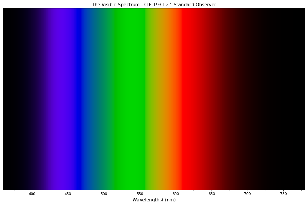
visible_spectrum_plot()
Overview
Colour is organised around various sub-packages:
- adaptation: Chromatic adaptation models and transformations.
- algebra: Algebra utilities.
- appearance: Colour appearance models.
- biochemistry: Biochemistry computations.
- continuous: Base objects for continuous data representation.
- characterisation: Colour fitting and camera characterisation.
- colorimetry: Core objects for colour computations.
- constants: CIE and CODATA constants.
- corresponding: Corresponding colour chromaticities computations.
- difference: Colour difference computations.
- examples: Examples for the sub-packages.
- io: Input / output objects for reading and writing data.
- models: Colour models.
- notation: Colour notation systems.
- phenomena: Computation of various optical phenomena.
- plotting: Diagrams, figures, etc…
- quality: Colour quality computation.
- recovery: Reflectance recovery.
- temperature: Colour temperature and correlated colour temperature computation.
- utilities: Various utilities and data structures.
- volume: Colourspace volumes computation and optimal colour stimuli.
Most of the public API is available from the root colour namespace:
import colour

print(colour.__all__[:5] + ['...'])
['handle_numpy_errors', 'ignore_numpy_errors', 'raise_numpy_errors', 'print_numpy_errors', 'warn_numpy_errors', '...']
The various sub-packages also expose their public API:
from pprint import pprint

import colour.plotting

for sub_package in ('adaptation', 'algebra', 'appearance', 'biochemistry',
                    'characterisation', 'colorimetry', 'constants',
                    'continuous', 'corresponding', 'difference', 'io',
                    'models', 'notation', 'phenomena', 'plotting', 'quality',
                    'recovery', 'temperature', 'utilities', 'volume'):
    print(sub_package.title())
    pprint(getattr(colour, sub_package).__all__[:5] + ['...'])
    print('\n')
Adaptation
['CHROMATIC_ADAPTATION_TRANSFORMS',
 'XYZ_SCALING_CAT',
 'VON_KRIES_CAT',
 'BRADFORD_CAT',
 'SHARP_CAT',
 '...']


Algebra
['cartesian_to_spherical',
 'spherical_to_cartesian',
 'cartesian_to_polar',
 'polar_to_cartesian',
 'cartesian_to_cylindrical',
 '...']


Appearance
['Hunt_InductionFactors',
 'HUNT_VIEWING_CONDITIONS',
 'Hunt_Specification',
 'XYZ_to_Hunt',
 'ATD95_Specification',
 '...']


Biochemistry
['reaction_rate_MichealisMenten',
 'substrate_concentration_MichealisMenten',
 '...']


Characterisation
['RGB_SpectralSensitivities',
 'RGB_DisplayPrimaries',
 'CAMERAS_RGB_SPECTRAL_SENSITIVITIES',
 'COLOURCHECKERS',
 'COLOURCHECKER_INDEXES_TO_NAMES_MAPPING',
 '...']


Colorimetry
['SpectralShape',
 'SpectralPowerDistribution',
 'MultiSpectralPowerDistribution',
 'DEFAULT_SPECTRAL_SHAPE',
 'constant_spd',
 '...']


Continuous
['AbstractContinuousFunction', 'Signal', 'MultiSignal', '...']


Constants
['CIE_E', 'CIE_K', 'K_M', 'KP_M', 'AVOGADRO_CONSTANT', '...']


Corresponding
['BRENEMAN_EXPERIMENTS',
 'BRENEMAN_EXPERIMENTS_PRIMARIES_CHROMATICITIES',
 'corresponding_chromaticities_prediction_CIE1994',
 'corresponding_chromaticities_prediction_CMCCAT2000',
 'corresponding_chromaticities_prediction_Fairchild1990',
 '...']


Difference
['DELTA_E_METHODS',
 'delta_E',
 'delta_E_CIE1976',
 'delta_E_CIE1994',
 'delta_E_CIE2000',
 '...']


Io
['IES_TM2714_Spd',
 'read_image',
 'write_image',
 'read_spectral_data_from_csv_file',
 'read_spds_from_csv_file',
 '...']


Models
['XYZ_to_xyY', 'xyY_to_XYZ', 'xy_to_xyY', 'xyY_to_xy', 'xy_to_XYZ', '...']


Notation
['MUNSELL_COLOURS_ALL',
 'MUNSELL_COLOURS_1929',
 'MUNSELL_COLOURS_REAL',
 'MUNSELL_COLOURS',
 'munsell_value',
 '...']


Phenomena
['scattering_cross_section',
 'rayleigh_optical_depth',
 'rayleigh_scattering',
 'rayleigh_scattering_spd',
 '...']


Plotting
['ASTM_G_173_ETR',
 'PLOTTING_RESOURCES_DIRECTORY',
 'DEFAULT_FIGURE_ASPECT_RATIO',
 'DEFAULT_FIGURE_WIDTH',
 'DEFAULT_FIGURE_HEIGHT',
 '...']


Quality
['TCS_SPDS',
 'VS_SPDS',
 'CRI_Specification',
 'colour_rendering_index',
 'CQS_Specification',
 '...']


Recovery
['SMITS_1999_SPDS',
 'XYZ_to_spectral_Meng2015',
 'RGB_to_spectral_Smits1999',
 'REFLECTANCE_RECOVERY_METHODS',
 'XYZ_to_spectral',
 '...']


Temperature
['CCT_TO_UV_METHODS',
 'UV_TO_CCT_METHODS',
 'CCT_to_uv',
 'CCT_to_uv_Ohno2013',
 'CCT_to_uv_Robertson1968',
 '...']


Utilities
['handle_numpy_errors',
 'ignore_numpy_errors',
 'raise_numpy_errors',
 'print_numpy_errors',
 'warn_numpy_errors',
 '...']


Volume
['ILLUMINANTS_OPTIMAL_COLOUR_STIMULI',
 'is_within_macadam_limits',
 'is_within_mesh_volume',
 'is_within_pointer_gamut',
 'is_within_visible_spectrum',
 '...']
The code is documented and almost every docstrings have usage examples:
print(colour.temperature.CCT_to_uv_Ohno2013.__doc__)
Returns the *CIE UCS* colourspace *uv* chromaticity coordinates from given
correlated colour temperature :math:`T_{cp}`, :math:`\Delta_{uv}` and
colour matching functions using *Ohno (2013)* method.

Parameters
----------
CCT : numeric
    Correlated colour temperature :math:`T_{cp}`.
D_uv : numeric, optional
    :math:`\Delta_{uv}`.
cmfs : XYZ_ColourMatchingFunctions, optional
    Standard observer colour matching functions.

Returns
-------
ndarray
    *CIE UCS* colourspace *uv* chromaticity coordinates.

References
----------
.. [4]  Ohno, Y. (2014). Practical Use and Calculation of CCT and Duv.
        LEUKOS, 10(1), 47–55. doi:10.1080/15502724.2014.839020

Examples
--------
>>> from colour import STANDARD_OBSERVERS_CMFS
>>> cmfs = STANDARD_OBSERVERS_CMFS['CIE 1931 2 Degree Standard Observer']
>>> CCT = 6507.4342201047066
>>> D_uv = 0.003223690901513
>>> CCT_to_uv_Ohno2013(CCT, D_uv, cmfs)  # doctest: +ELLIPSIS
array([ 0.1977999...,  0.3122004...])
At the core of Colour is
the colour.colorimetry sub-package, it defines the objects needed
for spectral related computations and many others:
import colour.colorimetry as colorimetry

pprint(colorimetry.__all__)
['SpectralShape',
 'SpectralPowerDistribution',
 'MultiSpectralPowerDistribution',
 'DEFAULT_SPECTRAL_SHAPE',
 'constant_spd',
 'zeros_spd',
 'ones_spd',
 'blackbody_spd',
 'blackbody_spectral_radiance',
 'planck_law',
 'LMS_ConeFundamentals',
 'RGB_ColourMatchingFunctions',
 'XYZ_ColourMatchingFunctions',
 'CMFS',
 'LMS_CMFS',
 'RGB_CMFS',
 'STANDARD_OBSERVERS_CMFS',
 'ILLUMINANTS',
 'D_ILLUMINANTS_S_SPDS',
 'HUNTERLAB_ILLUMINANTS',
 'ILLUMINANTS_RELATIVE_SPDS',
 'LIGHT_SOURCES',
 'LIGHT_SOURCES_RELATIVE_SPDS',
 'LEFS',
 'PHOTOPIC_LEFS',
 'SCOTOPIC_LEFS',
 'BANDPASS_CORRECTION_METHODS',
 'bandpass_correction',
 'bandpass_correction_Stearns1988',
 'D_illuminant_relative_spd',
 'CIE_standard_illuminant_A_function',
 'mesopic_luminous_efficiency_function',
 'mesopic_weighting_function',
 'LIGHTNESS_METHODS',
 'lightness',
 'lightness_Glasser1958',
 'lightness_Wyszecki1963',
 'lightness_CIE1976',
 'lightness_Fairchild2010',
 'lightness_Fairchild2011',
 'LUMINANCE_METHODS',
 'luminance',
 'luminance_Newhall1943',
 'luminance_ASTMD153508',
 'luminance_CIE1976',
 'luminance_Fairchild2010',
 'luminance_Fairchild2011',
 'dominant_wavelength',
 'complementary_wavelength',
 'excitation_purity',
 'colorimetric_purity',
 'luminous_flux',
 'luminous_efficiency',
 'luminous_efficacy',
 'RGB_10_degree_cmfs_to_LMS_10_degree_cmfs',
 'RGB_2_degree_cmfs_to_XYZ_2_degree_cmfs',
 'RGB_10_degree_cmfs_to_XYZ_10_degree_cmfs',
 'LMS_2_degree_cmfs_to_XYZ_2_degree_cmfs',
 'LMS_10_degree_cmfs_to_XYZ_10_degree_cmfs',
 'SPECTRAL_TO_XYZ_METHODS',
 'spectral_to_XYZ',
 'ASTME30815_PRACTISE_SHAPE',
 'lagrange_coefficients_ASTME202211',
 'tristimulus_weighting_factors_ASTME202211',
 'adjust_tristimulus_weighting_factors_ASTME30815',
 'spectral_to_XYZ_integration',
 'spectral_to_XYZ_tristimulus_weighting_factors_ASTME30815',
 'spectral_to_XYZ_ASTME30815',
 'wavelength_to_XYZ',
 'WHITENESS_METHODS',
 'whiteness',
 'whiteness_Berger1959',
 'whiteness_Taube1960',
 'whiteness_Stensby1968',
 'whiteness_ASTME313',
 'whiteness_Ganz1979',
 'whiteness_CIE2004',
 'YELLOWNESS_METHODS',
 'yellowness',
 'yellowness_ASTMD1925',
 'yellowness_ASTME313']
Colour computations
leverage a comprehensive dataset available in pretty much each
sub-packages, for example colour.colorimetry.dataset defines the
following data:
import colour.colorimetry.dataset as dataset

pprint(dataset.__all__)
['CMFS',
 'LMS_CMFS',
 'RGB_CMFS',
 'STANDARD_OBSERVERS_CMFS',
 'ILLUMINANTS',
 'D_ILLUMINANTS_S_SPDS',
 'HUNTERLAB_ILLUMINANTS',
 'ILLUMINANTS_RELATIVE_SPDS',
 'LIGHT_SOURCES',
 'LIGHT_SOURCES_RELATIVE_SPDS',
 'LEFS',
 'PHOTOPIC_LEFS',
 'SCOTOPIC_LEFS']
From Spectral Power Distribution
Whether it be a sample spectral power distribution, colour matching
functions or illuminants, spectral data is manipulated using an object
built with the colour.SpectralPowerDistribution class or based on
it:
# Defining a sample spectral power distribution data.
sample_spd_data = {
    380: 0.048,
    385: 0.051,
    390: 0.055,
    395: 0.060,
    400: 0.065,
    405: 0.068,
    410: 0.068,
    415: 0.067,
    420: 0.064,
    425: 0.062,
    430: 0.059,
    435: 0.057,
    440: 0.055,
    445: 0.054,
    450: 0.053,
    455: 0.053,
    460: 0.052,
    465: 0.052,
    470: 0.052,
    475: 0.053,
    480: 0.054,
    485: 0.055,
    490: 0.057,
    495: 0.059,
    500: 0.061,
    505: 0.062,
    510: 0.065,
    515: 0.067,
    520: 0.070,
    525: 0.072,
    530: 0.074,
    535: 0.075,
    540: 0.076,
    545: 0.078,
    550: 0.079,
    555: 0.082,
    560: 0.087,
    565: 0.092,
    570: 0.100,
    575: 0.107,
    580: 0.115,
    585: 0.122,
    590: 0.129,
    595: 0.134,
    600: 0.138,
    605: 0.142,
    610: 0.146,
    615: 0.150,
    620: 0.154,
    625: 0.158,
    630: 0.163,
    635: 0.167,
    640: 0.173,
    645: 0.180,
    650: 0.188,
    655: 0.196,
    660: 0.204,
    665: 0.213,
    670: 0.222,
    675: 0.231,
    680: 0.242,
    685: 0.251,
    690: 0.261,
    695: 0.271,
    700: 0.282,
    705: 0.294,
    710: 0.305,
    715: 0.318,
    720: 0.334,
    725: 0.354,
    730: 0.372,
    735: 0.392,
    740: 0.409,
    745: 0.420,
    750: 0.436,
    755: 0.450,
    760: 0.462,
    765: 0.465,
    770: 0.448,
    775: 0.432,
    780: 0.421}

spd = colour.SpectralPowerDistribution(sample_spd_data, name='Sample')
print(repr(spd))
SpectralPowerDistribution([[  3.80000000e+02,   4.80000000e-02],
                           [  3.85000000e+02,   5.10000000e-02],
                           [  3.90000000e+02,   5.50000000e-02],
                           [  3.95000000e+02,   6.00000000e-02],
                           [  4.00000000e+02,   6.50000000e-02],
                           [  4.05000000e+02,   6.80000000e-02],
                           [  4.10000000e+02,   6.80000000e-02],
                           [  4.15000000e+02,   6.70000000e-02],
                           [  4.20000000e+02,   6.40000000e-02],
                           [  4.25000000e+02,   6.20000000e-02],
                           [  4.30000000e+02,   5.90000000e-02],
                           [  4.35000000e+02,   5.70000000e-02],
                           [  4.40000000e+02,   5.50000000e-02],
                           [  4.45000000e+02,   5.40000000e-02],
                           [  4.50000000e+02,   5.30000000e-02],
                           [  4.55000000e+02,   5.30000000e-02],
                           [  4.60000000e+02,   5.20000000e-02],
                           [  4.65000000e+02,   5.20000000e-02],
                           [  4.70000000e+02,   5.20000000e-02],
                           [  4.75000000e+02,   5.30000000e-02],
                           [  4.80000000e+02,   5.40000000e-02],
                           [  4.85000000e+02,   5.50000000e-02],
                           [  4.90000000e+02,   5.70000000e-02],
                           [  4.95000000e+02,   5.90000000e-02],
                           [  5.00000000e+02,   6.10000000e-02],
                           [  5.05000000e+02,   6.20000000e-02],
                           [  5.10000000e+02,   6.50000000e-02],
                           [  5.15000000e+02,   6.70000000e-02],
                           [  5.20000000e+02,   7.00000000e-02],
                           [  5.25000000e+02,   7.20000000e-02],
                           [  5.30000000e+02,   7.40000000e-02],
                           [  5.35000000e+02,   7.50000000e-02],
                           [  5.40000000e+02,   7.60000000e-02],
                           [  5.45000000e+02,   7.80000000e-02],
                           [  5.50000000e+02,   7.90000000e-02],
                           [  5.55000000e+02,   8.20000000e-02],
                           [  5.60000000e+02,   8.70000000e-02],
                           [  5.65000000e+02,   9.20000000e-02],
                           [  5.70000000e+02,   1.00000000e-01],
                           [  5.75000000e+02,   1.07000000e-01],
                           [  5.80000000e+02,   1.15000000e-01],
                           [  5.85000000e+02,   1.22000000e-01],
                           [  5.90000000e+02,   1.29000000e-01],
                           [  5.95000000e+02,   1.34000000e-01],
                           [  6.00000000e+02,   1.38000000e-01],
                           [  6.05000000e+02,   1.42000000e-01],
                           [  6.10000000e+02,   1.46000000e-01],
                           [  6.15000000e+02,   1.50000000e-01],
                           [  6.20000000e+02,   1.54000000e-01],
                           [  6.25000000e+02,   1.58000000e-01],
                           [  6.30000000e+02,   1.63000000e-01],
                           [  6.35000000e+02,   1.67000000e-01],
                           [  6.40000000e+02,   1.73000000e-01],
                           [  6.45000000e+02,   1.80000000e-01],
                           [  6.50000000e+02,   1.88000000e-01],
                           [  6.55000000e+02,   1.96000000e-01],
                           [  6.60000000e+02,   2.04000000e-01],
                           [  6.65000000e+02,   2.13000000e-01],
                           [  6.70000000e+02,   2.22000000e-01],
                           [  6.75000000e+02,   2.31000000e-01],
                           [  6.80000000e+02,   2.42000000e-01],
                           [  6.85000000e+02,   2.51000000e-01],
                           [  6.90000000e+02,   2.61000000e-01],
                           [  6.95000000e+02,   2.71000000e-01],
                           [  7.00000000e+02,   2.82000000e-01],
                           [  7.05000000e+02,   2.94000000e-01],
                           [  7.10000000e+02,   3.05000000e-01],
                           [  7.15000000e+02,   3.18000000e-01],
                           [  7.20000000e+02,   3.34000000e-01],
                           [  7.25000000e+02,   3.54000000e-01],
                           [  7.30000000e+02,   3.72000000e-01],
                           [  7.35000000e+02,   3.92000000e-01],
                           [  7.40000000e+02,   4.09000000e-01],
                           [  7.45000000e+02,   4.20000000e-01],
                           [  7.50000000e+02,   4.36000000e-01],
                           [  7.55000000e+02,   4.50000000e-01],
                           [  7.60000000e+02,   4.62000000e-01],
                           [  7.65000000e+02,   4.65000000e-01],
                           [  7.70000000e+02,   4.48000000e-01],
                           [  7.75000000e+02,   4.32000000e-01],
                           [  7.80000000e+02,   4.21000000e-01]],
                          interpolator=SpragueInterpolator,
                          interpolator_args={},
                          extrapolator=Extrapolator,
                          extrapolator_args={u'right': None, u'method': u'Constant', u'left': None})
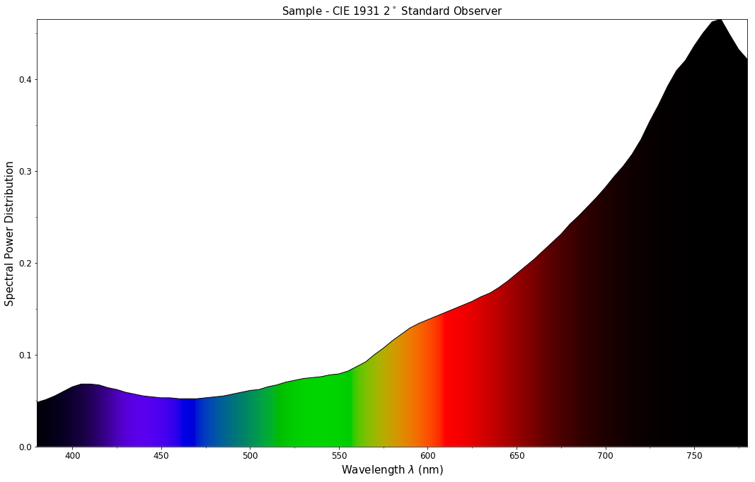
The sample spectral power distribution can be easily plotted against the visible spectrum:
# Plotting the sample spectral power distribution.
single_spd_plot(spd)
With the sample spectral power distribution defined, we can retrieve its shape:
# Displaying the sample spectral power distribution shape.
print(spd.shape)
(380.0, 780.0, 5.0)
The shape returned is an instance of colour.SpectralShape class:
repr(spd.shape)
'SpectralShape(380.0, 780.0, 5.0)'
colour.SpectralShape is used throughout
Colour to define
spectral dimensions and is instantiated as follows:
# Using *colour.SpectralShape* with iteration.
shape = colour.SpectralShape(start=0, end=10, interval=1)
for wavelength in shape:
    print(wavelength)

# *colour.SpectralShape.range* method is providing the complete range of values.
shape = colour.SpectralShape(0, 10, 0.5)
shape.range()
0.0
1.0
2.0
3.0
4.0
5.0
6.0
7.0
8.0
9.0
10.0
array([  0. ,   0.5,   1. ,   1.5,   2. ,   2.5,   3. ,   3.5,   4. ,
         4.5,   5. ,   5.5,   6. ,   6.5,   7. ,   7.5,   8. ,   8.5,
         9. ,   9.5,  10. ])
Colour defines three convenient objects to create constant spectral power distributions:
colour.constant_spdcolour.zeros_spdcolour.ones_spd
# Defining a constant spectral power distribution.
constant_spd = colour.constant_spd(100)
print('"Constant Spectral Power Distribution"')
print(constant_spd.shape)
print(constant_spd[400])

# Defining a zeros filled spectral power distribution.
print('\n"Zeros Filled Spectral Power Distribution"')
zeros_spd = colour.zeros_spd()
print(zeros_spd.shape)
print(zeros_spd[400])

# Defining a ones filled spectral power distribution.
print('\n"Ones Filled Spectral Power Distribution"')
ones_spd = colour.ones_spd()
print(ones_spd.shape)
print(ones_spd[400])
"Constant Spectral Power Distribution"
(360.0, 780.0, 1.0)
100.0

"Zeros Filled Spectral Power Distribution"
(360.0, 780.0, 1.0)
0.0

"Ones Filled Spectral Power Distribution"
(360.0, 780.0, 1.0)
1.0
By default the shape used by colour.constant_spd,
colour.zeros_spd and colour.ones_spd is the one defined by
colour.DEFAULT_SPECTRAL_SHAPE attribute using the CIE 1931 2°
Standard Observer shape.
print(repr(colour.DEFAULT_SPECTRAL_SHAPE))
SpectralShape(360, 780, 1)
A custom shape can be passed to construct a constant spectral power distribution with user defined dimensions:
colour.ones_spd(colour.SpectralShape(400, 700, 5))[450]
1.0
The colour.SpectralPowerDistribution class supports the following
arithmetical operations:
- addition
- subtraction
- multiplication
- division
spd1 = colour.ones_spd()
print('"Ones Filled Spectral Power Distribution"')
print(spd1[400])

print('\n"x2 Constant Multiplied"')
print((spd1 * 2)[400])

print('\n"+ Spectral Power Distribution"')
print((spd1 + colour.ones_spd())[400])
"Ones Filled Spectral Power Distribution"
1.0

"x2 Constant Multiplied"
2.0

"+ Spectral Power Distribution"
2.0
Often interpolation of the spectral power distribution is needed, this
is achieved with the colour.SpectralPowerDistribution.interpolate
method. Depending on the wavelengths uniformity, the default
interpolation method will differ. Following CIE 167:2005
recommendation: The method developed by Sprague (1880) should be used
for interpolating functions having a uniformly spaced independent
variable and a Cubic Spline method for non-uniformly spaced
independent variable [CIET13805a].
We can check the uniformity of the sample spectral power distribution:
# Checking the sample spectral power distribution uniformity.
print(spd.is_uniform())
True
Since the sample spectral power distribution is uniform the
interpolation will default to the colour.SpragueInterpolator
interpolator.
Note
Interpolation happens in place and may alter your original
data, use the colour.SpectralPowerDistribution.copy method to
produce a copy of your spectral power distribution before
interpolation.
# *Colour* can emit a substantial amount of warnings, we filter them.
colour.filter_warnings()
# Copying the sample spectral power distribution.
spd_copy = spd.copy()
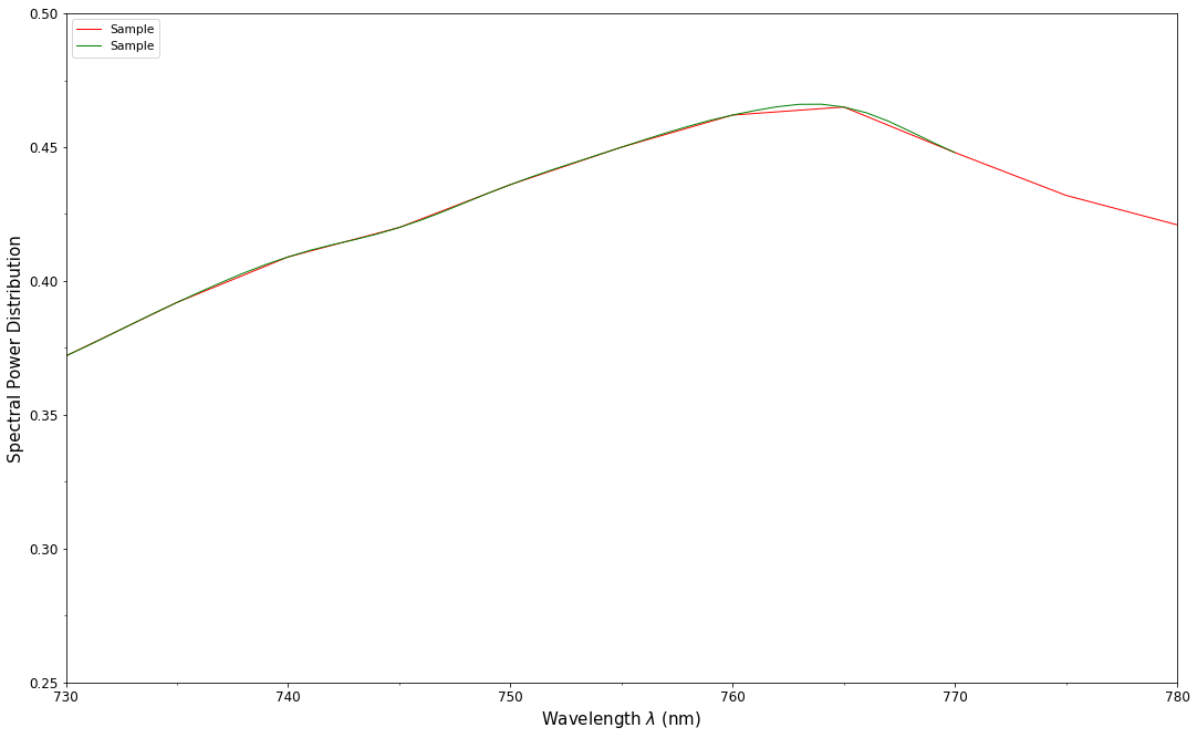
# Interpolating the copied sample spectral power distribution.
spd_copy.interpolate(colour.SpectralShape(400, 770, 1))
spd_copy[401]
0.065809599999999996
# Comparing the interpolated spectral power distribution with the original one.
multi_spd_plot([spd, spd_copy], bounding_box=[730,780, 0.25, 0.5])
Extrapolation although dangerous can be used to help aligning two spectral power distributions together. CIE publication CIE 15:2004 “Colorimetry” recommends that unmeasured values may be set equal to the nearest measured value of the appropriate quantity in truncation [CIET14804d]:
# Extrapolating the copied sample spectral power distribution.
spd_copy.extrapolate(colour.SpectralShape(340, 830))
spd_copy[340], spd_copy[830]
(0.065000000000000002, 0.44800000000000018)
The underlying interpolator can be swapped for any of the Colour interpolators.
pprint([
    export for export in colour.algebra.interpolation.__all__
    if 'Interpolator' in export
])
[u'KernelInterpolator',
 u'LinearInterpolator',
 u'SpragueInterpolator',
 u'CubicSplineInterpolator',
 u'PchipInterpolator',
 u'NullInterpolator']
# Changing interpolator while trimming the copied spectral power distribution.
spd_copy.interpolate(
    colour.SpectralShape(400, 700, 10), interpolator=colour.LinearInterpolator)
SpectralPowerDistribution([[  4.00000000e+02,   6.50000000e-02],
                           [  4.10000000e+02,   6.80000000e-02],
                           [  4.20000000e+02,   6.40000000e-02],
                           [  4.30000000e+02,   5.90000000e-02],
                           [  4.40000000e+02,   5.50000000e-02],
                           [  4.50000000e+02,   5.30000000e-02],
                           [  4.60000000e+02,   5.20000000e-02],
                           [  4.70000000e+02,   5.20000000e-02],
                           [  4.80000000e+02,   5.40000000e-02],
                           [  4.90000000e+02,   5.70000000e-02],
                           [  5.00000000e+02,   6.10000000e-02],
                           [  5.10000000e+02,   6.50000000e-02],
                           [  5.20000000e+02,   7.00000000e-02],
                           [  5.30000000e+02,   7.40000000e-02],
                           [  5.40000000e+02,   7.60000000e-02],
                           [  5.50000000e+02,   7.90000000e-02],
                           [  5.60000000e+02,   8.70000000e-02],
                           [  5.70000000e+02,   1.00000000e-01],
                           [  5.80000000e+02,   1.15000000e-01],
                           [  5.90000000e+02,   1.29000000e-01],
                           [  6.00000000e+02,   1.38000000e-01],
                           [  6.10000000e+02,   1.46000000e-01],
                           [  6.20000000e+02,   1.54000000e-01],
                           [  6.30000000e+02,   1.63000000e-01],
                           [  6.40000000e+02,   1.73000000e-01],
                           [  6.50000000e+02,   1.88000000e-01],
                           [  6.60000000e+02,   2.04000000e-01],
                           [  6.70000000e+02,   2.22000000e-01],
                           [  6.80000000e+02,   2.42000000e-01],
                           [  6.90000000e+02,   2.61000000e-01],
                           [  7.00000000e+02,   2.82000000e-01]],
                          interpolator=SpragueInterpolator,
                          interpolator_args={},
                          extrapolator=Extrapolator,
                          extrapolator_args={u'right': None, u'method': u'Constant', u'left': None})
The extrapolation behaviour can be changed for Linear method instead of the Constant default method or even use arbitrary constant left and right values:
# Extrapolating the copied sample spectral power distribution with *Linear* method.
spd_copy.extrapolate(
    colour.SpectralShape(340, 830),
    extrapolator_args={'method': 'Linear',
                       'right': 0})
spd_copy[340], spd_copy[830]
(0.046999999999999348, 0.0)
Aligning a spectral power distribution is a convenient way to first interpolates the current data within its original bounds, then, if required, extrapolate any missing values to match the requested shape:
# Aligning the cloned sample spectral power distribution.
# We first trim the spectral power distribution as above.
spd_copy.interpolate(colour.SpectralShape(400, 700))
spd_copy.align(colour.SpectralShape(340, 830, 5))
spd_copy[340], spd_copy[830]
(0.065000000000000002, 0.28199999999999975)
The colour.SpectralPowerDistribution class also supports various
arithmetic operations like addition, subtraction, multiplication
or division with numeric and array_like variables or other
colour.SpectralPowerDistribution class instances:
spd = colour.SpectralPowerDistribution({
    410: 0.25,
    420: 0.50,
    430: 0.75,
    440: 1.0,
    450: 0.75,
    460: 0.50,
    480: 0.25
})

print((spd.copy() + 1).values)
print((spd.copy() * 2).values)
print((spd * [0.35, 1.55, 0.75, 2.55, 0.95, 0.65, 0.15]).values)
print((spd * colour.constant_spd(2, spd.shape) * colour.constant_spd(3, spd.shape)).values)
[ 1.25  1.5   1.75  2.    1.75  1.5   1.25]
[ 0.5  1.   1.5  2.   1.5  1.   0.5]
[ 0.0875  0.775   0.5625  2.55    0.7125  0.325   0.0375]
[ 1.5  3.   4.5  6.   4.5  3.   nan  1.5]
The spectral power distribution can be normalised with an arbitrary factor:
print(spd.normalise().values)
print(spd.normalise(100).values)
[ 0.25  0.5   0.75  1.    0.75  0.5   0.25]
[  25.   50.   75.  100.   75.   50.   25.]
A the heart of the colour.SpectralPowerDistribution class is the
colour.continuous.Signal class which implements the
colour.continuous.Signal.function method.
Evaluating the function for any independent domain \(x \in \mathbb{R}\) variable returns a corresponding range \(y \in \mathbb{R}\) variable.
It adopts an interpolating function encapsulated inside an extrapolating
function. The resulting function independent domain, stored as discrete
values in the colour.continuous.Signal.domain attribute corresponds
with the function dependent and already known range stored in the
colour.continuous.Signal.range attribute.
Describing the colour.continuous.Signal class is beyond the scope of
this tutorial but we can illustrate its core capability.
import numpy as np

range_ = np.linspace(10, 100, 10)
signal = colour.continuous.Signal(range_)
print(repr(signal))
Signal([[   0.,   10.],
        [   1.,   20.],
        [   2.,   30.],
        [   3.,   40.],
        [   4.,   50.],
        [   5.,   60.],
        [   6.,   70.],
        [   7.,   80.],
        [   8.,   90.],
        [   9.,  100.]],
       interpolator=KernelInterpolator,
       interpolator_args={},
       extrapolator=Extrapolator,
       extrapolator_args={u'right': nan, u'method': u'Constant', u'left': nan})
# Returning the corresponding range *y* variable for any arbitrary independent domain *x* variable.
signal[np.random.uniform(0, 9, 10)]
array([ 55.91309735,  65.4172615 ,  65.54495059,  88.17819416,
        61.88860248,  10.53878826,  55.25130534,  46.14659783,
        86.41406136,  84.59897703])
Convert to Tristimulus Values
From a given spectral power distribution, CIE XYZ tristimulus values can be calculated:
spd = colour.SpectralPowerDistribution(sample_spd_data)
cmfs = colour.STANDARD_OBSERVERS_CMFS['CIE 1931 2 Degree Standard Observer']
illuminant = colour.ILLUMINANTS_RELATIVE_SPDS['D65']

# Calculating the sample spectral power distribution *CIE XYZ* tristimulus values.
XYZ = colour.spectral_to_XYZ(spd, cmfs, illuminant)
print(XYZ)
[ 10.97085572 9.70278591 6.05562778]
From CIE XYZ Colourspace
CIE XYZ is the central colourspace for Colour Science from which many computations are available, cascading to even more computations:
# Displaying objects interacting directly with the *CIE XYZ* colourspace.
pprint([name for name in colour.__all__ if name.startswith('XYZ_to')])
['XYZ_to_Hunt',
 'XYZ_to_ATD95',
 'XYZ_to_CIECAM02',
 'XYZ_to_LLAB',
 'XYZ_to_Nayatani95',
 'XYZ_to_RLAB',
 'XYZ_to_xyY',
 'XYZ_to_xy',
 'XYZ_to_Lab',
 'XYZ_to_Luv',
 'XYZ_to_UCS',
 'XYZ_to_UVW',
 'XYZ_to_hdr_CIELab',
 'XYZ_to_K_ab_HunterLab1966',
 'XYZ_to_Hunter_Lab',
 'XYZ_to_Hunter_Rdab',
 'XYZ_to_Hunter_Rdab',
 'XYZ_to_IPT',
 'XYZ_to_hdr_IPT',
 'XYZ_to_colourspace_model',
 'XYZ_to_RGB',
 'XYZ_to_sRGB',
 'XYZ_to_spectral_Meng2015',
 'XYZ_to_spectral']
Convert to Screen Colours
We can for instance converts the CIE XYZ tristimulus values into sRGB colourspace RGB values in order to display them on screen:
# The output domain of *colour.spectral_to_XYZ* is [0, 100] and the input
# domain of *colour.XYZ_to_sRGB* is [0, 1]. We need to take it in account and
# rescale the input *CIE XYZ* colourspace matrix.
RGB = colour.XYZ_to_sRGB(XYZ / 100)
print(RGB)
[ 0.45675795 0.30986982 0.24861924]
# Plotting the *sRGB* colourspace colour of the *Sample* spectral power distribution.
single_colour_swatch_plot(ColourSwatch('Sample', RGB), text_size=32)
Generate Colour Rendition Charts
In the same way, we can compute values from a colour rendition chart sample.
Note
This is useful for render time checks in the VFX industry, where you can use a synthetic colour chart into your render and ensure the colour management is acting as expected.
The colour.characterisation sub-package contains the dataset for
various colour rendition charts:
# Colour rendition charts chromaticity coordinates.
print(sorted(colour.characterisation.COLOURCHECKERS.keys()))

# Colour rendition charts spectral power distributions.
print(sorted(colour.characterisation.COLOURCHECKERS_SPDS.keys()))
[u'BabelColor Average', u'ColorChecker 1976', u'ColorChecker 2005', u'babel_average', u'cc2005']
[u'BabelColor Average', u'ColorChecker N Ohta', u'babel_average', u'cc_ohta']
Note
The above cc2005, babel_average and cc_ohta keys are convenient aliases for respectively ColorChecker 2005, BabelColor Average and ColorChecker N Ohta keys.
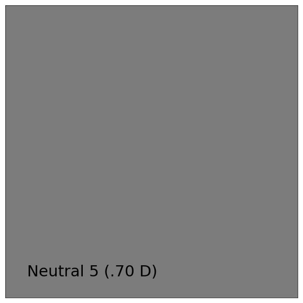
# Plotting the *sRGB* colourspace colour of *neutral 5 (.70 D)* patch.
patch_name = 'neutral 5 (.70 D)'
patch_spd = colour.COLOURCHECKERS_SPDS['ColorChecker N Ohta'][patch_name]
XYZ = colour.spectral_to_XYZ(patch_spd, cmfs, illuminant)
RGB = colour.XYZ_to_sRGB(XYZ / 100)

single_colour_swatch_plot(ColourSwatch(patch_name.title(), RGB), text_size=32)
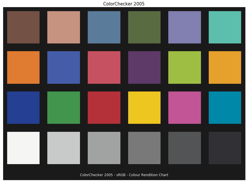
Colour defines a convenient plotting object to draw synthetic colour rendition charts figures:
colour_checker_plot(colour_checker='ColorChecker 2005', text_display=False)
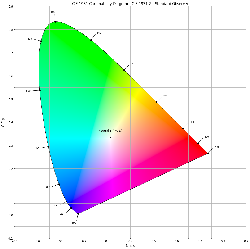
Convert to Chromaticity Coordinates
Given a spectral power distribution, chromaticity coordinates xy can
be computed using the colour.XYZ_to_xy definition:
# Computing *xy* chromaticity coordinates for the *neutral 5 (.70 D)* patch.
xy =  colour.XYZ_to_xy(XYZ)
print(xy)
[ 0.31259787 0.32870029]
Chromaticity coordinates xy can be plotted into the CIE 1931 Chromaticity Diagram:
import pylab

# Plotting the *CIE 1931 Chromaticity Diagram*.
# The argument *standalone=False* is passed so that the plot doesn't get displayed
# and can be used as a basis for other plots.
chromaticity_diagram_plot_CIE1931(standalone=False)

# Plotting the *xy* chromaticity coordinates.
x, y = xy
pylab.plot(x, y, 'o-', color='white')

# Annotating the plot.
pylab.annotate(patch_spd.name.title(),
               xy=xy,
               xytext=(-50, 30),
               textcoords='offset points',
               arrowprops=dict(arrowstyle='->', connectionstyle='arc3, rad=-0.2'))

# Displaying the plot.
render(
    standalone=True,
    limits=(-0.1, 0.9, -0.1, 0.9),
    x_tighten=True,
    y_tighten=True)
And More…
We hope that this small introduction has been useful and gave you the envy to see more, if you want to explore the API a good place to start is the Jupyter Notebooks page.