Basic Usage#
This page puts an emphasis on basic concepts of Colour, those are important to understand.
Object Name Categorisation#
The API tries to bundle the objects by categories by naming them with common prefixes which makes introspection and auto-completion easier.
For example, in IPython or Jupyter Notebook, most of the definitions pertaining to the spectral distribution handling can be found as follows:
In [1]: import colour

In [2]: colour.sd_
 sd_blackbody()                            sd_gaussian()                             sd_rayleigh_scattering()                  sd_zeros
 sd_CIE_illuminant_D_series()              sd_mesopic_luminous_efficiency_function() sd_single_led()
 sd_CIE_standard_illuminant_A()            sd_multi_leds()                           sd_to_aces_relative_exposure_values()
 sd_constant()                             sd_ones()                                 sd_to_XYZ
Likewise, for the spectral distribution handling related attributes:
In [2]: colour.SD
                  SD_GAUSSIAN_METHODS   SD_TO_XYZ_METHODS     SDS_ILLUMINANTS       SDS_LIGHT_SOURCES
                  SD_MULTI_LEDS_METHODS SDS_COLOURCHECKERS    SDS_LEFS
                  SD_SINGLE_LED_METHODS SDS_FILTERS           SDS_LENSES
Similarly, all the RGB colourspaces can be individually accessed from the
colour.models namespace:
In [2]: colour.models.RGB_COLOURSPACE
                         RGB_COLOURSPACE_ACES2065_1           RGB_COLOURSPACE_ACESPROXY            RGB_COLOURSPACE_APPLE_RGB            RGB_COLOURSPACE_BT470_525
                         RGB_COLOURSPACE_ACESCC               RGB_COLOURSPACE_ADOBE_RGB1998        RGB_COLOURSPACE_BEST_RGB             RGB_COLOURSPACE_BT470_625
                         RGB_COLOURSPACE_ACESCCT              RGB_COLOURSPACE_ADOBE_WIDE_GAMUT_RGB RGB_COLOURSPACE_BETA_RGB             RGB_COLOURSPACE_BT709                >
                         RGB_COLOURSPACE_ACESCG               RGB_COLOURSPACE_ARRI_WIDE_GAMUT_3    RGB_COLOURSPACE_BT2020               RGB_COLOURSPACE_CIE_RGB
Abbreviations#
The following abbreviations are in use in Colour:
CAM : Colour Appearance Model
CCS : Chromaticity Coordinates
CCTF : Colour Component Transfer Function
CCT : Correlated Colour Temperature
CMY : Cyan, Magenta, Yellow
CMYK : Cyan, Magenta, Yellow, Black
CVD : Colour Vision Deficiency
CV : Code Value
EOTF : Electro-Optical Transfer Function
IDT : Input Device Transform
MSDS : Multi-Spectral Distributions
OETF : Optical-Electrical Transfer Function
OOTF : Optical-Optical Transfer Function
SD : Spectral Distribution
TVS : Tristimulus Values
N-Dimensional Array Support#
Most of Colour definitions are fully vectorised and support n-dimensional array by leveraging Numpy.
While it is recommended to use ndarray as input for the API objects, it is possible to use tuples or lists:
import colour

xyY = (0.4316, 0.3777, 0.1008)
colour.xyY_to_XYZ(xyY)
array([ 0.11518475, 0.1008 , 0.05089373])
xyY = [0.4316, 0.3777, 0.1008]
colour.xyY_to_XYZ(xyY)
array([ 0.11518475, 0.1008 , 0.05089373])
xyY = [
    (0.4316, 0.3777, 0.1008),
    (0.4316, 0.3777, 0.1008),
    (0.4316, 0.3777, 0.1008),
]
colour.xyY_to_XYZ(xyY)
array([[ 0.11518475,  0.1008    ,  0.05089373],
       [ 0.11518475,  0.1008    ,  0.05089373],
       [ 0.11518475,  0.1008    ,  0.05089373]])
As shown in the above example, there is widespread support for n-dimensional arrays:
import numpy as np

xyY = np.array([0.4316, 0.3777, 0.1008])
xyY = np.tile(xyY, (6, 1))
colour.xyY_to_XYZ(xyY)
array([[ 0.11518475,  0.1008    ,  0.05089373],
       [ 0.11518475,  0.1008    ,  0.05089373],
       [ 0.11518475,  0.1008    ,  0.05089373],
       [ 0.11518475,  0.1008    ,  0.05089373],
       [ 0.11518475,  0.1008    ,  0.05089373],
       [ 0.11518475,  0.1008    ,  0.05089373]])
colour.xyY_to_XYZ(xyY.reshape([2, 3, 3]))
array([[[ 0.11518475,  0.1008    ,  0.05089373],
        [ 0.11518475,  0.1008    ,  0.05089373],
        [ 0.11518475,  0.1008    ,  0.05089373]],

       [[ 0.11518475,  0.1008    ,  0.05089373],
        [ 0.11518475,  0.1008    ,  0.05089373],
        [ 0.11518475,  0.1008    ,  0.05089373]]])
Which enables image processing:
RGB = colour.read_image("_static/Logo_Small_001.png")
RGB = RGB[..., 0:3]  # Discarding alpha channel.
XYZ = colour.sRGB_to_XYZ(RGB)
colour.plotting.plot_image(XYZ, text_kwargs={"text": "sRGB to XYZ"})
Spectral Representation and Continuous Signal#
Floating Point Wavelengths#
Colour current representation of spectral data is atypical and has been influenced by the failures and shortcomings of the previous implementation that required less than ideal code to support floating point wavelengths. Wavelengths should not have to be defined as integer values and it is effectively common to get data from instruments whose domain is returned as floating point values.
For example, the data from an Ocean Insight (Optics) STS-VIS spectrometer is typically saved with 3 digits decimal precision:
Data from Subt2_14-36-15-210.txt Node

Date: Sat Nov 17 14:36:15 NZDT 2018
User: kelsolaar
Spectrometer: S12286
Trigger mode: 0
Resolution mode: 1024 pixels
Integration Time (sec): 5.000000E0
Scans to average: 3
Nonlinearity correction enabled: true
Boxcar width: 3
Baseline correction enabled: true
XAxis mode: Wavelengths
Number of Pixels in Spectrum: 1024
# >>>>>Begin Spectral Data<<<<<
338.028     279.71
338.482     285.43
338.936     291.33
...
821.513     3112.65
822.008     3133.74
822.503     3107.11
A solution to the problem is to quantize the data at integer values but it is often non-desirable. The spectra representation implementation prior to Colour 0.3.11 was relying on a custom mutable mapping which was allowing to retrieve decimal keys within a given precision:
data_1 = {0.1999999998: "Nemo", 0.2000000000: "John"}
apm_1 = ArbitraryPrecisionMapping(data_1, key_decimals=10)
tuple(apm_1.keys())
(0.1999999998, 0.2)
apm_2 = ArbitraryPrecisionMapping(data_1, key_decimals=7)
tuple(apm_2.keys())
(0.2,)
While functional, the approach was brittle and not elegant which triggered a significant amount of rework.
Continuous Signal#
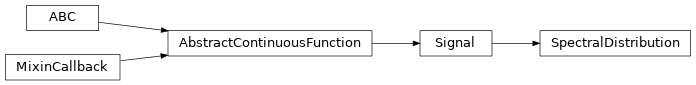
All the spectral distributions in Colour are instances of the
colour.SpectralDistribution class (or its sub-classes), a sub-class of
the colour.continuous.Signal class which is itself an implementation
of the colour.continuous.AbstractContinuousFunction ABCMeta
class:
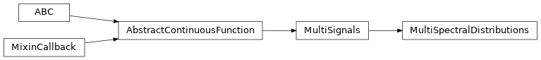
Likewise, the multi-spectral distributions are instances
colour.MultiSpectralDistributions class (or its sub-classes), a
sub-class of the colour.continuous.MultiSignals class which is a
container for multiple colour.continuous.Signal sub-class instances
and also implements the colour.continuous.AbstractContinuousFunction
ABCMeta class.
The colour.continuous.Signal class implements the
Signal.function() method so that evaluating the function for any
independent domain \(x \in\mathbb{R}\) variable returns a corresponding
range \(y \in\mathbb{R}\) variable.
It adopts an interpolating function encapsulated inside an extrapolating
function. The resulting function independent domain, stored as discrete values
in the colour.continuous.Signal.domain attribute corresponds with the
function dependent and already known range stored in the
colour.continuous.Signal.range attribute.
Consequently, it is possible to get the value of a spectral distribution at any given wavelength:
data = {
    500: 0.0651,
    520: 0.0705,
    540: 0.0772,
    560: 0.0870,
    580: 0.1128,
    600: 0.1360,
}
sd = colour.SpectralDistribution(data)
sd[555.5]
0.083453673782958995
Getting, Setting, Indexing and Slicing#
Attention
Indexing a spectral distribution (or multi-spectral distribution) with a numeric (or a numeric sequence) returns the corresponding value(s). Indexing a spectral distribution (or multi-spectral distribution) with a slice returns the values for the corresponding wavelength indexes.
While it is tempting to think that the colour.SpectralDistribution
and colour.MultiSpectralDistributions classes behave like Numpy’s
ndarray,
they do not entirely and some peculiarities exist that make them different.
An important difference lies in the behaviour with respect to getting and setting the values of the data.
Getting the value(s) for a single (or multiple wavelengths) is done by indexing
the colour.SpectralDistribution (or
colour.MultiSpectralDistributions) class with the a single numeric
or array of numeric wavelengths, e.g., sd[555.5] or
sd[555.25, 555.25, 555.75].
However, if getting the values using a slice class instance, e.g.,
sd[0:3], the underlying discrete values for the indexes represented by the
slice class instance are returned instead.
As shown in the previous section, getting the value of a wavelength is done as follows:
data = {
    500: 0.0651,
    520: 0.0705,
    540: 0.0772,
    560: 0.0870,
    580: 0.1128,
    600: 0.1360,
}
sd = colour.SpectralDistribution(data)
sd[555]
0.083135180664062502,
Multiple wavelength values can be retrieved as follows:
sd[(555.0, 556.25, 557.5, 558.75, 560.0)]
array([ 0.08313518, 0.08395997, 0.08488108, 0.085897 , 0.087 ])
However, slices will return the values for the corresponding wavelength indexes:
sd[0:3]
array([ 0.0651, 0.0705, 0.0772])
sd[:]
array([ 0.0651, 0.0705, 0.0772, 0.087 , 0.1128, 0.136 ])
Note
Indexing a multi-spectral distribution is achieved similarly, it can however be sliced along multiple axes because the data is2-dimensional, e.g., msds[0:3, 0:2].
A copy of the underlying colour.SpectralDistribution and
colour.MultiSpectralDistributions classes discretized data can be
accessed via the wavelengths and values properties. However, it cannot
be changed directly via the properties or slicing:
Attention
The data returned by the wavelengths and values properties is a
copy of the underlying colour.SpectralDistribution and
colour.MultiSpectralDistributions classes discretized data: It
can only be changed indirectly.
data = {
    500: 0.0651,
    520: 0.0705,
    540: 0.0772,
    560: 0.0870,
    580: 0.1128,
    600: 0.1360,
}
sd = colour.SpectralDistribution(data)
# Note: The wavelength 500nm is at index 0.
sd.values[0] = 0
sd[500]
0.065100000000000019
Instead, the values can be set indirectly:
values = sd.values
values[0] = 0
sd.values = values
sd.values
array([ 0. , 0.0705, 0.0772, 0.087 , 0.1128, 0.136 ])
Domain-Range Scales#
Note
This section contains important information.
Colour adopts 4 main input domains and output ranges:
Scalars usually in domain-range
[0, 1](or[0, 10]for Munsell Value).Percentages usually in domain-range
[0, 100].Degrees usually in domain-range
[0, 360].Integers usually in domain-range
[0, 2**n -1]wherenis the bit depth.
It is error prone but it is also a direct consequence of the inconsistency of
the colour science field itself. We have discussed at length about this and we
were leaning toward normalisation of the whole API to domain-range [0, 1],
we never committed for reasons highlighted by the following points:
Colour Scientist performing computations related to Munsell Renotation System would be very surprised if the output Munsell Value was in range
[0, 1]or[0, 100].A Visual Effect Industry artist would be astonished to find out that conversion from CIE XYZ to sRGB was yielding values in range
[0, 100].
However benefits of having a consistent and predictable domain-range scale are numerous thus with Colour 0.3.12 we have introduced a mechanism to allow users to work within one of the two available domain-range scales.
Scale - Reference#
‘Reference’ is the default domain-range scale of Colour, objects adopt the implemented reference, i.e., paper, publication, etc.., domain-range scale.
The ‘Reference’ domain-range scale is inconsistent, e.g., colour appearance
models, spectral conversions are typically in domain-range [0, 100] while RGB
models will operate in domain-range [0, 1]. Some objects, e.g.,
:func:colour.colorimetry.lightness_Fairchild2011 definition have mismatched
domain-range: input domain [0, 1] and output range [0, 100].
Scale - 1#
‘1’ is a domain-range scale converting all the relevant objects from
Colour public API to domain-range [0, 1]:
Scalars in domain-range
[0, 10], e.g Munsell Value are scaled by 10.Percentages in domain-range
[0, 100]are scaled by 100.Degrees in domain-range
[0, 360]are scaled by 360.Integers in domain-range
[0, 2**n -1]wherenis the bit depth are scaled by 2**n -1.Dimensionless values are unaffected and are indicated with
DN.Unaffected values are unaffected and are indicated with
UN.
Warning
The conversion to ‘1’ domain-range scale is a soft normalisation and
similarly to the ‘Reference’ domain-range scale it is normal to
encounter values exceeding 1, e.g., High Dynamic Range Imagery (HDRI) or
negative values, e.g., out-of-gamut RGB colourspace values. Some definitions
such as colour.models.eotf_ST2084() which decodes absolute luminance
values are not affected by any domain-range scales and are indicated with
UN.
Understanding the Domain-Range Scale of an Object#
Using colour.adaptation.chromatic_adaptation_CIE1994() definition
docstring as an example, the Notes section features two tables.
The first table is for the domain, and lists the input arguments affected by the two domain-range scales and which normalisation they should adopt depending the domain-range scale in use:
Domain |
Scale - Reference |
Scale - 1 |
|---|---|---|
|
[0, 100] |
[0, 1] |
|
[0, 100] |
[0, 1] |
The second table is for the range and lists the return value of the definition:
Range |
Scale - Reference |
Scale - 1 |
|---|---|---|
|
[0, 100] |
[0, 1] |
Working with the Domain-Range Scales#
The current domain-range scale is returned with the
colour.get_domain_range_scale() definition:
import colour

colour.get_domain_range_scale()
u'reference'
Changing from the ‘Reference’ default domain-range scale to ‘1’ is done
with the colour.set_domain_range_scale() definition:
XYZ_1 = [28.00, 21.26, 5.27]
xy_o1 = [0.4476, 0.4074]
xy_o2 = [0.3127, 0.3290]
Y_o = 20
E_o1 = 1000
E_o2 = 1000
colour.adaptation.chromatic_adaptation_CIE1994(XYZ_1, xy_o1, xy_o2, Y_o, E_o1, E_o2)
array([ 24.03379521, 21.15621214, 17.64301199])
colour.set_domain_range_scale("1")

XYZ_1 = [0.2800, 0.2126, 0.0527]
Y_o = 0.2
colour.adaptation.chromatic_adaptation_CIE1994(XYZ_1, xy_o1, xy_o2, Y_o, E_o1, E_o2)
array([ 0.24033795, 0.21156212, 0.17643012])
The output tristimulus values with the ‘1’ domain-range scale are equal to those from ‘Reference’ default domain-range scale divided by 100.
Passing incorrectly scaled values to the
colour.adaptation.chromatic_adaptation_CIE1994() definition
would result in unexpected values and a warning in that case:
colour.set_domain_range_scale("Reference")

colour.adaptation.chromatic_adaptation_CIE1994(XYZ_1, xy_o1, xy_o2, Y_o, E_o1, E_o2)
File "<ipython-input-...>", line 4, in <module>
  E_o2)
File "/colour-science/colour/colour/adaptation/cie1994.py", line 134, in chromatic_adaptation_CIE1994
  warning(('"Y_o" luminance factor must be in [18, 100] domain, '
/colour-science/colour/colour/utilities/verbose.py:207: ColourWarning: "Y_o" luminance factor must be in [18, 100] domain, unpredictable results may occur!
  warn(*args, **kwargs)
array([ 0.17171825,  0.13731098,  0.09972054])
Setting the ‘1’ domain-range scale has the following effect on the
colour.adaptation.chromatic_adaptation_CIE1994() definition:
As it expects values in domain [0, 100], scaling occurs and the
relevant input values, i.e., the values listed in the domain table, XYZ_1
and Y_o are converted from domain [0, 1] to domain [0, 100] by
colour.utilities.to_domain_100() definition and conversely
return value XYZ_2 is converted from range [0, 100] to range [0, 1]
by colour.utilities.from_range_100() definition.
A convenient alternative to the colour.set_domain_range_scale()
definition is the colour.domain_range_scale context manager and
decorator. It temporarily overrides Colour domain-range scale with given
scale value:
with colour.domain_range_scale("1"):
    colour.adaptation.chromatic_adaptation_CIE1994(XYZ_1, xy_o1, xy_o2, Y_o, E_o1, E_o2)
[ 0.24033795 0.21156212 0.17643012]
Multiprocessing on Windows with Domain-Range Scales#
Windows does not have a fork system call, a consequence is that child processes do not necessarily inherit from changes made to global variables.
It has crucial consequences as Colour stores the current domain-range scale into a global variable.
The solution is to define an initialisation definition that defines the scale upon child processes spawning.
The colour.utilities.multiprocessing_pool context manager conveniently
performs the required initialisation so that the domain-range scale is
propagated appropriately to child processes.
Safe Power and Division#
Colour default handling of fractional power and zero-division occurring during practical applications is managed via various definitions and context managers.
Safe Power#
NaNs generation occurs when a negative number \(a\) is raised to the
fractional power \(p\). This can be avoided using the
colour.algebra.spow() definition that raises to the power as follows:
\(sign(a) * |a|^p\).
To the extent possible, the colour.algebra.spow() definition has been
used throughout the codebase. The default behaviour is controlled with the
following definitions:
colour.algebra.set_spow_enabled()colour.algebra.spow_enable()(Context Manager & Decorator)
Safe Division#
NaNs and +/- infs generation occurs when a number \(a\) is divided 0. This
can be avoided using the colour.algebra.sdiv() definition. It has been
used wherever deemed relevant in the codebase. The default behaviour is
controlled with the following definitions:
colour.algebra.sdiv_mode()(Context Manager & Decorator)
The following modes are available:
Numpy: The current Numpy zero-division handling occurs.Ignore: Zero-division occurs silently.Warning: Zero-division occurs with a warning.Ignore Zero Conversion: Zero-division occurs silently and NaNs or +/- infs values are converted to zeros. Seenumpy.nan_to_num()definition for more details.Warning Zero Conversion: Zero-division occurs with a warning and NaNs or +/- infs values are converted to zeros. Seenumpy.nan_to_num()definition for more details.Ignore Limit Conversion: Zero-division occurs silently and NaNs or +/- infs values are converted to zeros or the largest +/- finite floating point values representable by the division resultnumpy.dtype. Seenumpy.nan_to_num()definition for more details.Warning Limit Conversion: Zero-division occurs with a warning and NaNs or +/- infs values are converted to zeros or the largest +/- finite floating point values representable by the division resultnumpy.dtype.
colour.algebra.get_sdiv_mode()
'Ignore Zero Conversion'
colour.algebra.set_sdiv_mode("Numpy")
colour.UCS_to_uv([0, 0, 0])
/Users/kelsolaar/Documents/Development/colour-science/colour/colour/algebra/common.py:317: RuntimeWarning: invalid value encountered in true_divide
  c = a / b
array([ nan,  nan])
colour.algebra.set_sdiv_mode("Ignore Zero Conversion")
colour.UCS_to_uv([0, 0, 0])
array([ 0., 0.])