Colour is an open-source Python package providing a comprehensive number of algorithms and datasets for colour science.
It is freely available under the New BSD License terms.
Colour is an affiliated project of NumFOCUS, a 501(c)(3) nonprofit in the United States.
Table of Contents
2 Sponsors
We are grateful for the support of our sponsors. If you’d like to join them, please consider becoming a sponsor on OpenCollective.
3 Features
Colour features a rich dataset and collection of objects, please see the features page for more information.
4 Installation
Colour can be easily installed from the Python Package Index by issuing this command in a shell:
$ pip install colour-science
Colour is also available for Anaconda from Continuum Analytics via conda-forge:
$ conda install -c conda-forge colour-science
The detailed installation procedure is described in the Installation Guide.
5 Documentation
5.1 Tutorial
The static tutorial provides an introduction to Colour. An interactive version is available via Google Colab.
5.2 How-To Guide
The How-To guide for Colour shows various techniques to solve specific problems and highlights some interesting use cases.
5.3 API Reference
The main technical reference for Colour and its API is the Colour Manual.
- Colour Manual
- Tutorial
- Basics
- Advanced
- Reference
- Colour
- Chromatic Adaptation
- Algebra
- Colour Appearance Models
- Biochemistry
- Colour Vision Deficiency
- Colour Characterisation
- Colorimetry
- Constants
- Contrast Sensitivity
- Continuous Signal
- Corresponding Chromaticities
- Colour Difference
- Automatic Colour Conversion Graph
- Input and Output
- Colour Models
- Colour Notation Systems
- Optical Phenomena
- Plotting
- Colour Quality
- Reflectance Recovery
- Colour Temperature
- Utilities
- Colour Volume
- Indices and tables
- Colour
- Bibliography
5.4 Jupyter Notebooks
Jupyter Notebooks are available and designed to provide an historical perspective of colour science via Colour usage.
5.5 Examples
Most of the objects are available from the colour namespace:
>>> import colour
5.5.1 Automatic Colour Conversion Graph - colour.graph
Starting with version 0.3.14, Colour implements an automatic colour conversion graph enabling easier colour conversions.
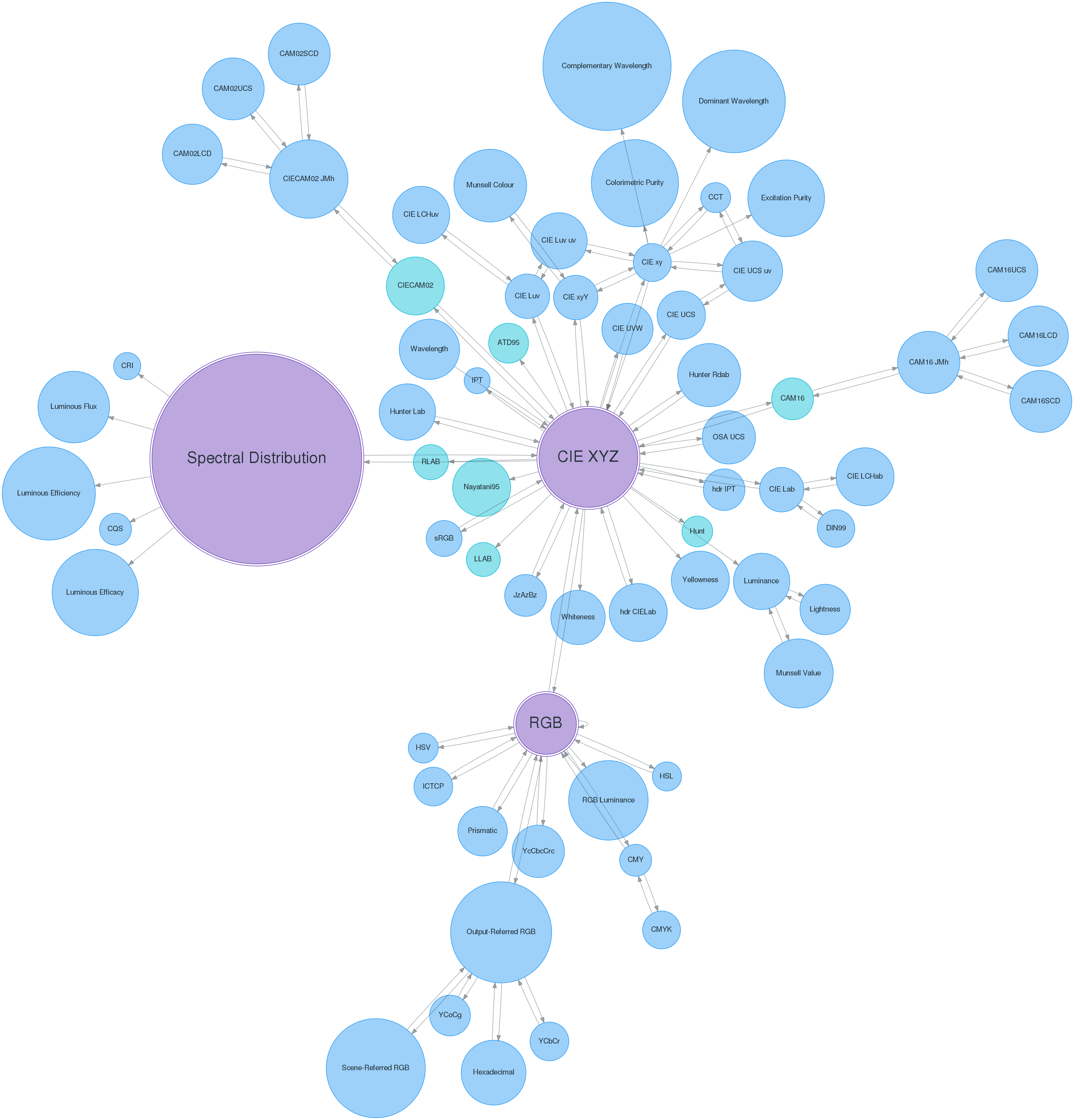
>>> sd = colour.COLOURCHECKERS_SDS['ColorChecker N Ohta']['dark skin']
>>> convert(sd, 'Spectral Distribution', 'sRGB', verbose={'mode': 'Short'})
===============================================================================
*                                                                             *
*   [ Conversion Path ]                                                       *
*                                                                             *
*   "sd_to_XYZ" --> "XYZ_to_sRGB"                                             *
*                                                                             *
===============================================================================
array([ 0.45675795,  0.30986982,  0.24861924])
>>> illuminant = colour.ILLUMINANTS_SDS['FL2']
>>> convert(sd, 'Spectral Distribution', 'sRGB', sd_to_XYZ={'illuminant': illuminant})
array([ 0.47924575,  0.31676968,  0.17362725])
5.5.2 Chromatic Adaptation - colour.adaptation
>>> XYZ = [0.20654008, 0.12197225, 0.05136952]
>>> D65 = colour.ILLUMINANTS['CIE 1931 2 Degree Standard Observer']['D65']
>>> A = colour.ILLUMINANTS['CIE 1931 2 Degree Standard Observer']['A']
>>> colour.chromatic_adaptation(
...     XYZ, colour.xy_to_XYZ(D65), colour.xy_to_XYZ(A))
array([ 0.2533053 ,  0.13765138,  0.01543307])
>>> sorted(colour.CHROMATIC_ADAPTATION_METHODS.keys())
['CIE 1994', 'CMCCAT2000', 'Fairchild 1990', 'Von Kries']
5.5.3 Algebra - colour.algebra
5.5.3.1 Kernel Interpolation
>>> y = [5.9200, 9.3700, 10.8135, 4.5100, 69.5900, 27.8007, 86.0500]
>>> x = range(len(y))
>>> colour.KernelInterpolator(x, y)([0.25, 0.75, 5.50])
array([  6.18062083,   8.08238488,  57.85783403])
5.5.3.2 Sprague (1880) Interpolation
>>> y = [5.9200, 9.3700, 10.8135, 4.5100, 69.5900, 27.8007, 86.0500]
>>> x = range(len(y))
>>> colour.SpragueInterpolator(x, y)([0.25, 0.75, 5.50])
array([  6.72951612,   7.81406251,  43.77379185])
5.5.4 Colour Appearance Models - colour.appearance
>>> XYZ = [0.20654008 * 100, 0.12197225 * 100, 0.05136952 * 100]
>>> XYZ_w = [95.05, 100.00, 108.88]
>>> L_A = 318.31
>>> Y_b = 20.0
>>> colour.XYZ_to_CIECAM02(XYZ, XYZ_w, L_A, Y_b)
CIECAM02_Specification(J=34.434525727858997, C=67.365010921125915, h=22.279164147957076, s=62.814855853327131, Q=177.47124941102123, M=70.024939419291385, H=2.689608534423904, HC=None)
5.5.5 Colour Blindness - colour.blindness
>>> import colour
>>> cmfs = colour.LMS_CMFS['Stockman & Sharpe 2 Degree Cone Fundamentals']
>>> colour.anomalous_trichromacy_cmfs_Machado2009(cmfs, np.array([15, 0, 0]))[450]
array([ 0.08912884,  0.0870524 ,  0.955393  ])
>>> primaries = colour.DISPLAYS_RGB_PRIMARIES['Apple Studio Display']
>>> d_LMS = (15, 0, 0)
>>> colour.anomalous_trichromacy_matrix_Machado2009(cmfs, primaries, d_LMS)
array([[-0.27774652,  2.65150084, -1.37375432],
       [ 0.27189369,  0.20047862,  0.52762768],
       [ 0.00644047,  0.25921579,  0.73434374]])
5.5.6 Colour Correction - colour characterisation
>>> import numpy as np
>>> RGB = [0.17224810, 0.09170660, 0.06416938]
>>> M_T = np.random.random((24, 3))
>>> M_R = M_T + (np.random.random((24, 3)) - 0.5) * 0.5
>>> colour.colour_correction(RGB, M_T, M_R)
array([ 0.15205429,  0.08974029,  0.04141435])
>>> sorted(colour.COLOUR_CORRECTION_METHODS.keys())
['Cheung 2004', 'Finlayson 2015', 'Vandermonde']
5.5.7 Colorimetry - colour.colorimetry
5.5.7.1 Spectral Computations
>>> colour.sd_to_XYZ(colour.LIGHT_SOURCES_SDS['Neodimium Incandescent'])
array([ 36.94726204,  32.62076174,  13.0143849 ])
>>> sorted(colour.SPECTRAL_TO_XYZ_METHODS.keys())
['ASTM E308', 'Integration', 'astm2015']
5.5.7.2 Multi-Spectral Computations
>>> msds = np.array([
...     [[0.01367208, 0.09127947, 0.01524376, 0.02810712, 0.19176012, 0.04299992],
...      [0.00959792, 0.25822842, 0.41388571, 0.22275120, 0.00407416, 0.37439537],
...      [0.01791409, 0.29707789, 0.56295109, 0.23752193, 0.00236515, 0.58190280]],
...     [[0.01492332, 0.10421912, 0.02240025, 0.03735409, 0.57663846, 0.32416266],
...      [0.04180972, 0.26402685, 0.03572137, 0.00413520, 0.41808194, 0.24696727],
...      [0.00628672, 0.11454948, 0.02198825, 0.39906919, 0.63640803, 0.01139849]],
...     [[0.04325933, 0.26825359, 0.23732357, 0.05175860, 0.01181048, 0.08233768],
...      [0.02484169, 0.12027161, 0.00541695, 0.00654612, 0.18603799, 0.36247808],
...      [0.03102159, 0.16815442, 0.37186235, 0.08610666, 0.00413520, 0.78492409]],
...     [[0.11682307, 0.78883040, 0.74468607, 0.83375293, 0.90571451, 0.70054168],
...      [0.06321812, 0.41898224, 0.15190357, 0.24591440, 0.55301750, 0.00657664],
...      [0.00305180, 0.11288624, 0.11357290, 0.12924391, 0.00195315, 0.21771573]],
... ])
>>> colour.multi_sds_to_XYZ(msds, cmfs, illuminant, method='Integration',
...                         shape=colour.SpectralShape(400, 700, 60)))
[[[  9.73192501   5.02105851   3.22790699]
  [ 16.08032168  24.47303359  10.28681006]
  [ 17.73513774  29.61865582  12.10713449]]
 [[ 25.69298792  11.72611193   3.70187275]
  [ 18.51208526   8.03720984   9.30361825]
  [ 48.55945054  32.30885571   4.09223401]]
 [[  5.7743232   10.10692925  10.08461311]
  [  8.81306527   3.65394599   4.20783881]
  [  8.06007398  15.87077693   7.02551086]]
 [[ 90.88877129  81.82966846  29.86765971]
  [ 38.64801062  26.70860262  15.08396538]
  [  8.77151115  10.56330761   4.28940206]]]
>>> sorted(colour.MULTI_SPECTRAL_TO_XYZ_METHODS.keys())
['ASTM E308', 'Integration', 'astm2015']
5.5.7.3 Blackbody Spectral Radiance Computation
>>> colour.sd_blackbody(5000)
SpectralDistribution([[  3.60000000e+02,   6.65427827e+12],
                      [  3.61000000e+02,   6.70960528e+12],
                      [  3.62000000e+02,   6.76482512e+12],
                      ...
                      [  7.78000000e+02,   1.06068004e+13],
                      [  7.79000000e+02,   1.05903327e+13],
                      [  7.80000000e+02,   1.05738520e+13]],
                     interpolator=SpragueInterpolator,
                     interpolator_args={},
                     extrapolator=Extrapolator,
                     extrapolator_args={'right': None, 'method': 'Constant', 'left': None})
5.5.7.4 Dominant, Complementary Wavelength & Colour Purity Computation
>>> xy = [0.54369557, 0.32107944]
>>> xy_n = [0.31270000, 0.32900000]
>>> colour.dominant_wavelength(xy, xy_n)
(array(616.0),
 array([ 0.68354746,  0.31628409]),
 array([ 0.68354746,  0.31628409]))
5.5.7.5 Lightness Computation
>>> colour.lightness(12.19722535)
41.527875844653451
>>> sorted(colour.LIGHTNESS_METHODS.keys())
['CIE 1976',
 'Fairchild 2010',
 'Fairchild 2011',
 'Glasser 1958',
 'Lstar1976',
 'Wyszecki 1963']
5.5.7.6 Luminance Computation
>>> colour.luminance(41.52787585)
12.197225353400775
>>> sorted(colour.LUMINANCE_METHODS.keys())
['ASTM D1535',
 'CIE 1976',
 'Fairchild 2010',
 'Fairchild 2011',
 'Newhall 1943',
 'astm2008',
 'cie1976']
5.5.7.7 Whiteness Computation
>>> XYZ = [95.00000000, 100.00000000, 105.00000000]
>>> XYZ_0 = [94.80966767, 100.00000000, 107.30513595]
>>> colour.whiteness(XYZ, XYZ_0)
array([ 93.756     ,  -1.33000001])
>>> sorted(colour.WHITENESS_METHODS.keys())
['ASTM E313',
 'Berger 1959',
 'CIE 2004',
 'Ganz 1979',
 'Stensby 1968',
 'Taube 1960',
 'cie2004']
5.5.7.8 Yellowness Computation
>>> XYZ = [95.00000000, 100.00000000, 105.00000000]
>>> colour.yellowness(XYZ)
11.065000000000003
>>> sorted(colour.YELLOWNESS_METHODS.keys())
['ASTM D1925', 'ASTM E313']
5.5.7.9 Luminous Flux, Efficiency & Efficacy Computation
>>> sd = colour.LIGHT_SOURCES_SDS['Neodimium Incandescent']
>>> colour.luminous_flux(sd)
23807.655527367202
>>> sd = colour.LIGHT_SOURCES_SDS['Neodimium Incandescent']
>>> colour.luminous_efficiency(sd)
0.19943935624521045
>>> sd = colour.LIGHT_SOURCES_SDS['Neodimium Incandescent']
>>> colour.luminous_efficacy(sd)
136.21708031547874
5.5.8 Contrast Sensitivity Function - colour.contrast
>>> colour.contrast_sensitivity_function(u=4, X_0=60, E=65)
358.51180789884984
>>> sorted(colour.CONTRAST_SENSITIVITY_METHODS.keys())
['Barten 1999']
5.5.9 Colour Difference - colour.difference
>>> Lab_1 = [100.00000000, 21.57210357, 272.22819350]
>>> Lab_2 = [100.00000000, 426.67945353, 72.39590835]
>>> colour.delta_E(Lab_1, Lab_2)
94.035649026659485
>>> sorted(colour.DELTA_E_METHODS.keys())
['CAM02-LCD',
 'CAM02-SCD',
 'CAM02-UCS',
 'CAM16-LCD',
 'CAM16-SCD',
 'CAM16-UCS',
 'CIE 1976',
 'CIE 1994',
 'CIE 2000',
 'CMC',
 'DIN99',
 'cie1976',
 'cie1994',
 'cie2000']
5.5.10 IO - colour.io
5.5.10.1 Images
>>> RGB = colour.read_image('Ishihara_Colour_Blindness_Test_Plate_3.png')
>>> RGB.shape
(276, 281, 3)
5.5.10.2 Look Up Table (LUT) Data
>>> LUT = colour.read_LUT('ACES_Proxy_10_to_ACES.cube')
>>> print(LUT)
LUT3x1D - ACES Proxy 10 to ACES
-------------------------------
Dimensions : 2
Domain     : [[0 0 0]
              [1 1 1]]
Size       : (32, 3)
>>> RGB = [0.17224810, 0.09170660, 0.06416938]
>>> LUT.apply(RGB)
array([ 0.00575674,  0.00181493,  0.00121419])
5.5.11 Colour Models - colour.models
5.5.11.1 CIE xyY Colourspace
>>> colour.XYZ_to_xyY([0.20654008, 0.12197225, 0.05136952])
array([ 0.54369557,  0.32107944,  0.12197225])
5.5.11.2 CIE L*a*b* Colourspace
>>> colour.XYZ_to_Lab([0.20654008, 0.12197225, 0.05136952])
array([ 41.52787529,  52.63858304,  26.92317922])
5.5.11.3 CIE L*u*v* Colourspace
>>> colour.XYZ_to_Luv([0.20654008, 0.12197225, 0.05136952])
array([ 41.52787529,  96.83626054,  17.75210149])
5.5.11.4 CIE 1960 UCS Colourspace
>>> colour.XYZ_to_UCS([0.20654008, 0.12197225, 0.05136952])
array([ 0.13769339,  0.12197225,  0.1053731 ])
5.5.11.5 CIE 1964 U*V*W* Colourspace
>>> XYZ = [0.20654008 * 100, 0.12197225 * 100, 0.05136952* 100]
>>> colour.XYZ_to_UVW(XYZ)
array([ 94.55035725,  11.55536523,  40.54757405])
5.5.11.6 Hunter L,a,b Colour Scale
>>> XYZ = [0.20654008 * 100, 0.12197225 * 100, 0.05136952* 100]
>>> colour.XYZ_to_Hunter_Lab(XYZ)
array([ 34.92452577,  47.06189858,  14.38615107])
5.5.11.7 Hunter Rd,a,b Colour Scale
>>> XYZ = [0.20654008 * 100, 0.12197225 * 100, 0.05136952* 100]
>>> colour.XYZ_to_Hunter_Rdab(XYZ)
array([ 12.197225  ,  57.12537874,  17.46241341])
5.5.11.8 CAM02-LCD, CAM02-SCD, and CAM02-UCS Colourspaces - Luo, Cui and Li (2006)
>>> XYZ = [0.20654008 * 100, 0.12197225 * 100, 0.05136952* 100]
>>> XYZ_w = [95.05, 100.00, 108.88]
>>> L_A = 318.31
>>> Y_b = 20.0
>>> surround = colour.CIECAM02_VIEWING_CONDITIONS['Average']
>>> specification = colour.XYZ_to_CIECAM02(
        XYZ, XYZ_w, L_A, Y_b, surround)
>>> JMh = (specification.J, specification.M, specification.h)
>>> colour.JMh_CIECAM02_to_CAM02UCS(JMh)
array([ 47.16899898,  38.72623785,  15.8663383 ])
5.5.11.9 CAM16-LCD, CAM16-SCD, and CAM16-UCS Colourspaces - Li et al. (2017)
>>> XYZ = [0.20654008 * 100, 0.12197225 * 100, 0.05136952* 100]
>>> XYZ_w = [95.05, 100.00, 108.88]
>>> L_A = 318.31
>>> Y_b = 20.0
>>> surround = colour.CAM16_VIEWING_CONDITIONS['Average']
>>> specification = colour.XYZ_to_CAM16(
        XYZ, XYZ_w, L_A, Y_b, surround)
>>> JMh = (specification.J, specification.M, specification.h)
>>> colour.JMh_CAM16_to_CAM16UCS(JMh)
array([ 46.55542238,  40.22460974,  14.25288392]
5.5.11.10 IPT Colourspace
>>> colour.XYZ_to_IPT([0.20654008, 0.12197225, 0.05136952])
array([ 0.38426191,  0.38487306,  0.18886838])
5.5.11.11 DIN99 Colourspace
>>> Lab = [41.52787529, 52.63858304, 26.92317922]
>>> colour.Lab_to_DIN99(Lab)
array([ 53.22821988,  28.41634656,   3.89839552])
5.5.11.12 hdr-CIELAB Colourspace
>>> colour.XYZ_to_hdr_CIELab([0.20654008, 0.12197225, 0.05136952])
array([ 51.87002062,  60.4763385 ,  32.14551912])
5.5.11.13 hdr-IPT Colourspace
>>> colour.XYZ_to_hdr_IPT([0.20654008, 0.12197225, 0.05136952])
array([ 25.18261761, -22.62111297,   3.18511729])
5.5.11.14 OSA UCS Colourspace
>>> XYZ = [0.20654008 * 100, 0.12197225 * 100, 0.05136952* 100]
>>> colour.XYZ_to_OSA_UCS(XYZ)
array([-3.0049979 ,  2.99713697, -9.66784231])
5.5.11.15 JzAzBz Colourspace
>>> colour.XYZ_to_JzAzBz([0.20654008, 0.12197225, 0.05136952])
array([ 0.00535048,  0.00924302,  0.00526007])
5.5.11.16 Y’CbCr Colour Encoding
>>> colour.RGB_to_YCbCr([1.0, 1.0, 1.0])
array([ 0.92156863,  0.50196078,  0.50196078])
5.5.11.17 YCoCg Colour Encoding
>>> colour.RGB_to_YCoCg([0.75, 0.75, 0.0])
array([ 0.5625,  0.375 ,  0.1875])
5.5.11.18 ICTCP Colour Encoding
>>> colour.RGB_to_ICTCP([0.45620519, 0.03081071, 0.04091952])
array([ 0.07351364,  0.00475253,  0.09351596])
5.5.11.19 HSV Colourspace
>>> colour.RGB_to_HSV([0.45620519, 0.03081071, 0.04091952])
array([ 0.99603944,  0.93246304,  0.45620519])
5.5.11.20 Prismatic Colourspace
>>> colour.RGB_to_Prismatic([0.25, 0.50, 0.75])
array([ 0.75      ,  0.16666667,  0.33333333,  0.5       ])
5.5.11.21 RGB Colourspace and Transformations
>>> XYZ = [0.21638819, 0.12570000, 0.03847493]
>>> illuminant_XYZ = [0.34570, 0.35850]
>>> illuminant_RGB = [0.31270, 0.32900]
>>> chromatic_adaptation_transform = 'Bradford'
>>> XYZ_to_RGB_matrix = [
         [3.24062548, -1.53720797, -0.49862860],
         [-0.96893071, 1.87575606, 0.04151752],
         [0.05571012, -0.20402105, 1.05699594]]
>>> colour.XYZ_to_RGB(
         XYZ,
         illuminant_XYZ,
         illuminant_RGB,
         XYZ_to_RGB_matrix,
         chromatic_adaptation_transform)
array([ 0.45595571,  0.03039702,  0.04087245])
5.5.11.22 RGB Colourspace Derivation
>>> p = [0.73470, 0.26530, 0.00000, 1.00000, 0.00010, -0.07700]
>>> w = [0.32168, 0.33767]
>>> colour.normalised_primary_matrix(p, w)
array([[  9.52552396e-01,   0.00000000e+00,   9.36786317e-05],
       [  3.43966450e-01,   7.28166097e-01,  -7.21325464e-02],
       [  0.00000000e+00,   0.00000000e+00,   1.00882518e+00]])
5.5.11.23 RGB Colourspaces
>>> sorted(colour.RGB_COLOURSPACES.keys())
['ACES2065-1',
 'ACEScc',
 'ACEScct',
 'ACEScg',
 'ACESproxy',
 'ALEXA Wide Gamut',
 'Adobe RGB (1998)',
 'Adobe Wide Gamut RGB',
 'Apple RGB',
 'Best RGB',
 'Beta RGB',
 'CIE RGB',
 'Cinema Gamut',
 'ColorMatch RGB',
 'DCDM XYZ',
 'DCI-P3',
 'DCI-P3+',
 'Display P3',
 'DJI D-Gamut',
 'DRAGONcolor',
 'DRAGONcolor2',
 'Don RGB 4',
 'ECI RGB v2',
 'ERIMM RGB',
 'Ekta Space PS 5',
 'F-Gamut',
 'FilmLight E-Gamut',
 'ITU-R BT.2020',
 'ITU-R BT.470 - 525',
 'ITU-R BT.470 - 625',
 'ITU-R BT.709',
 'Max RGB',
 'NTSC (1953)',
 'NTSC (1987)',
 'P3-D65',
 'Pal/Secam',
 'ProPhoto RGB',
 'Protune Native',
 'REDWideGamutRGB',
 'REDcolor',
 'REDcolor2',
 'REDcolor3',
 'REDcolor4',
 'RIMM RGB',
 'ROMM RGB',
 'Russell RGB',
 'S-Gamut',
 'S-Gamut3',
 'S-Gamut3.Cine',
 'SMPTE 240M',
 'SMPTE C',
 'Sharp RGB',
 'V-Gamut',
 'Xtreme RGB',
 'aces',
 'adobe1998',
 'prophoto',
 'sRGB']
5.5.11.24 OETFs
>>> sorted(colour.OETFS.keys())
['ARIB STD-B67',
 'ITU-R BT.2020',
 'ITU-R BT.2100 HLG',
 'ITU-R BT.2100 PQ',
 'ITU-R BT.601',
 'ITU-R BT.709',
 'SMPTE 240M']
5.5.11.25 OETFs Inverse
>>> sorted(colour.OETF_INVERSES.keys())
['ARIB STD-B67',
 'ITU-R BT.2100 HLD',
 'ITU-R BT.2100 PQ',
 'ITU-R BT.601',
 'ITU-R BT.709']
5.5.11.26 EOTFs
>>> sorted(colour.EOTFS.keys())
['DCDM',
 'DICOM GSDF',
 'ITU-R BT.1886',
 'ITU-R BT.2020',
 'ITU-R BT.2100 HLG',
 'ITU-R BT.2100 PQ',
 'SMPTE 240M',
 'ST 2084',
 'sRGB']
5.5.11.27 EOTFs Inverse
>>> sorted(colour.EOTF_INVERSES.keys())
['DCDM',
 'DICOM GSDF',
 'ITU-R BT.1886',
 'ITU-R BT.2100 HLG',
 'ITU-R BT.2100 PQ',
 'ST 2084',
 'sRGB']
5.5.11.28 OOTFs
>>> sorted(colour.OOTFS.keys())
['ITU-R BT.2100 HLG', 'ITU-R BT.2100 PQ']
5.5.11.29 OOTFs Inverse
>>> sorted(colour.OOTF_INVERSES.keys())
['ITU-R BT.2100 HLG', 'ITU-R BT.2100 PQ']
5.5.11.30 Log Encoding / Decoding
>>> sorted(colour.LOG_ENCODINGS.keys())
['ACEScc',
 'ACEScct',
 'ACESproxy',
 'ALEXA Log C',
 'Canon Log',
 'Canon Log 2',
 'Canon Log 3',
 'Cineon',
 'D-Log',
 'ERIMM RGB',
 'F-Log',
 'Filmic Pro 6',
 'Log3G10',
 'Log3G12',
 'PLog',
 'Panalog',
 'Protune',
 'REDLog',
 'REDLogFilm',
 'S-Log',
 'S-Log2',
 'S-Log3',
 'T-Log',
 'V-Log',
 'ViperLog']
5.5.11.31 CCTFs Encoding / Decoding
>>> sorted(colour.CCTF_ENCODINGS.keys())
['ACEScc',
 'ACEScct',
 'ACESproxy',
 'ALEXA Log C',
 'ARIB STD-B67',
 'Canon Log',
 'Canon Log 2',
 'Canon Log 3',
 'Cineon',
 'D-Log',
 'DCDM',
 'DICOM GSDF',
 'ERIMM RGB',
 'F-Log',
 'Filmic Pro 6',
 'Gamma 2.2',
 'Gamma 2.4',
 'Gamma 2.6',
 'ITU-R BT.1886',
 'ITU-R BT.2020',
 'ITU-R BT.2100 HLG',
 'ITU-R BT.2100 PQ',
 'ITU-R BT.601',
 'ITU-R BT.709',
 'Log3G10',
 'Log3G12',
 'PLog',
 'Panalog',
 'ProPhoto RGB',
 'Protune',
 'REDLog',
 'REDLogFilm',
 'RIMM RGB',
 'ROMM RGB',
 'S-Log',
 'S-Log2',
 'S-Log3',
 'SMPTE 240M',
 'ST 2084',
 'T-Log',
 'V-Log',
 'ViperLog',
 'sRGB']
5.5.12 Colour Notation Systems - colour.notation
5.5.12.1 Munsell Value
>>> colour.munsell_value(12.23634268)
4.0824437076525664
>>> sorted(colour.MUNSELL_VALUE_METHODS.keys())
['ASTM D1535',
 'Ladd 1955',
 'McCamy 1987',
 'Moon 1943',
 'Munsell 1933',
 'Priest 1920',
 'Saunderson 1944',
 'astm2008']
5.5.12.2 Munsell Colour
>>> colour.xyY_to_munsell_colour([0.38736945, 0.35751656, 0.59362000])
'4.2YR 8.1/5.3'
>>> colour.munsell_colour_to_xyY('4.2YR 8.1/5.3')
array([ 0.38736945,  0.35751656,  0.59362   ])
5.5.13 Optical Phenomena - colour.phenomena
>>> colour.rayleigh_scattering_sd()
SpectralDistribution([[  3.60000000e+02,   5.99101337e-01],
                      [  3.61000000e+02,   5.92170690e-01],
                      [  3.62000000e+02,   5.85341006e-01],
                      ...
                      [  7.78000000e+02,   2.55208377e-02],
                      [  7.79000000e+02,   2.53887969e-02],
                      [  7.80000000e+02,   2.52576106e-02]],
                     interpolator=SpragueInterpolator,
                     interpolator_args={},
                     extrapolator=Extrapolator,
                     extrapolator_args={'right': None, 'method': 'Constant', 'left': None})
5.5.14 Light Quality - colour.quality
5.5.14.1 Colour Rendering Index
>>> colour.colour_quality_scale(colour.ILLUMINANTS_SDS['FL2'])
64.017283509280588
>>> colour.COLOUR_QUALITY_SCALE_METHODS
('NIST CQS 7.4', 'NIST CQS 9.0')
5.5.14.2 Colour Quality Scale
>>> colour.colour_rendering_index(colour.ILLUMINANTS_SDS['FL2'])
64.151520202968015
5.5.14.3 Academy Spectral Similarity Index (SSI)
>>> colour.spectral_similarity_index(colour.ILLUMINANTS_SDS['C'], colour.ILLUMINANTS_SDS['D65'])
94.0
5.5.15 Spectral Up-sampling & Reflectance Recovery - colour.recovery
>>> colour.XYZ_to_sd([0.20654008, 0.12197225, 0.05136952])
SpectralDistribution([[  3.60000000e+02,   7.73462151e-02],
                      [  3.65000000e+02,   7.73632975e-02],
                      [  3.70000000e+02,   7.74299705e-02],
                      ...
                      [  8.20000000e+02,   3.93126353e-01],
                      [  8.25000000e+02,   3.93158148e-01],
                      [  8.30000000e+02,   3.93163548e-01]],
                     interpolator=SpragueInterpolator,
                     interpolator_args={},
                     extrapolator=Extrapolator,
                     extrapolator_args={'right': None, 'method': 'Constant', 'left': None})

>>> sorted(colour.REFLECTANCE_RECOVERY_METHODS.keys())
['Meng 2015', 'Smits 1999']
5.5.17 Colour Volume - colour.volume
>>> colour.RGB_colourspace_volume_MonteCarlo(colour.RGB_COLOURSPACE['sRGB'])
821958.30000000005
5.5.18 Plotting - colour.plotting
Most of the objects are available from the colour.plotting namespace:
>>> from colour.plotting import *
>>> colour_style()
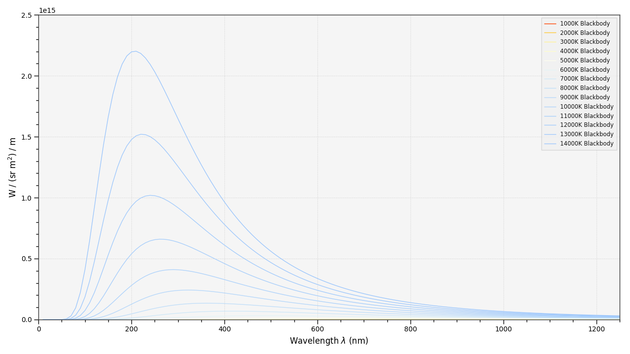
5.5.18.3 Blackbody
>>> blackbody_sds = [
...     colour.sd_blackbody(i, colour.SpectralShape(0, 10000, 10))
...     for i in range(1000, 15000, 1000)
... ]
>>> plot_multi_sds(
...     blackbody_sds,
...     y_label='W / (sr m$^2$) / m',
...     use_sds_colours=True,
...     normalise_sds_colours=True,
...     legend_location='upper right',
...     bounding_box=(0, 1250, 0, 2.5e15))
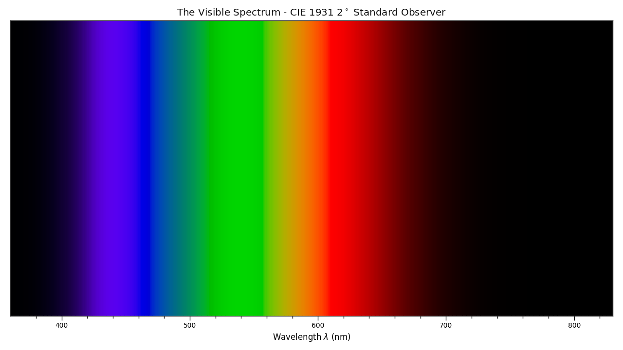
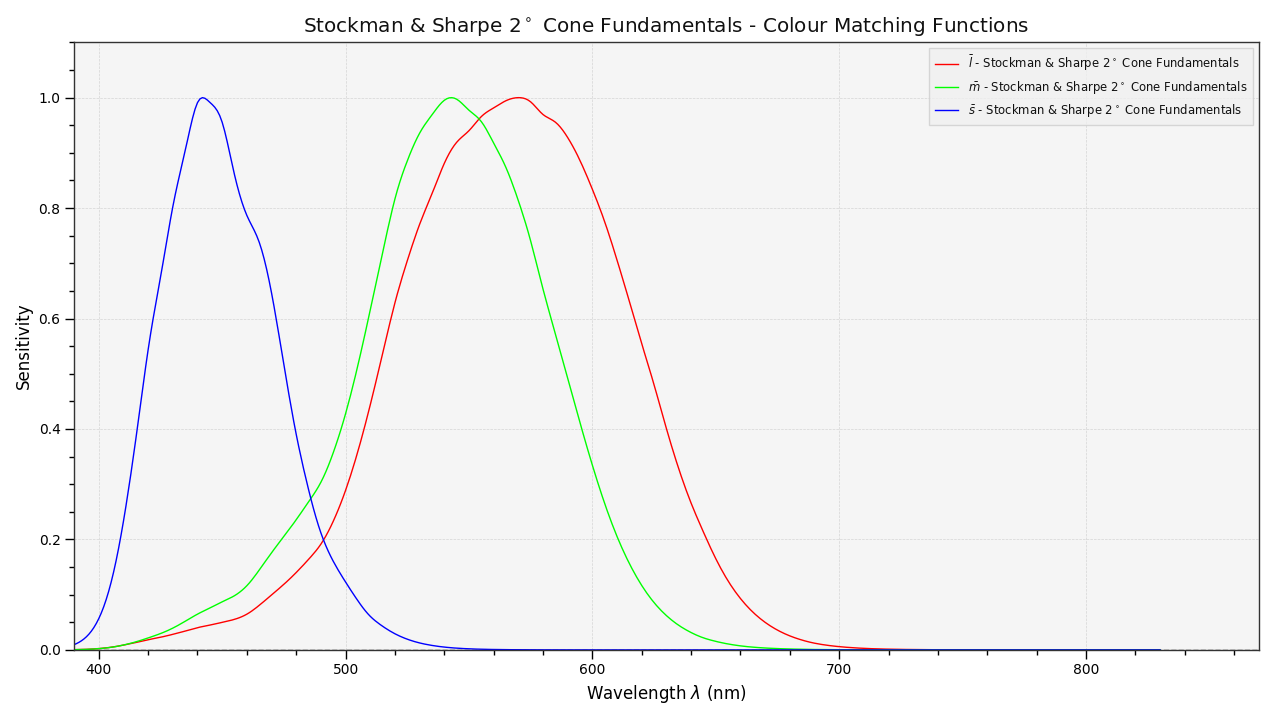
5.5.18.4 Colour Matching Functions
>>> plot_single_cmfs(
...     'Stockman & Sharpe 2 Degree Cone Fundamentals',
...     y_label='Sensitivity',
...     bounding_box=(390, 870, 0, 1.1))
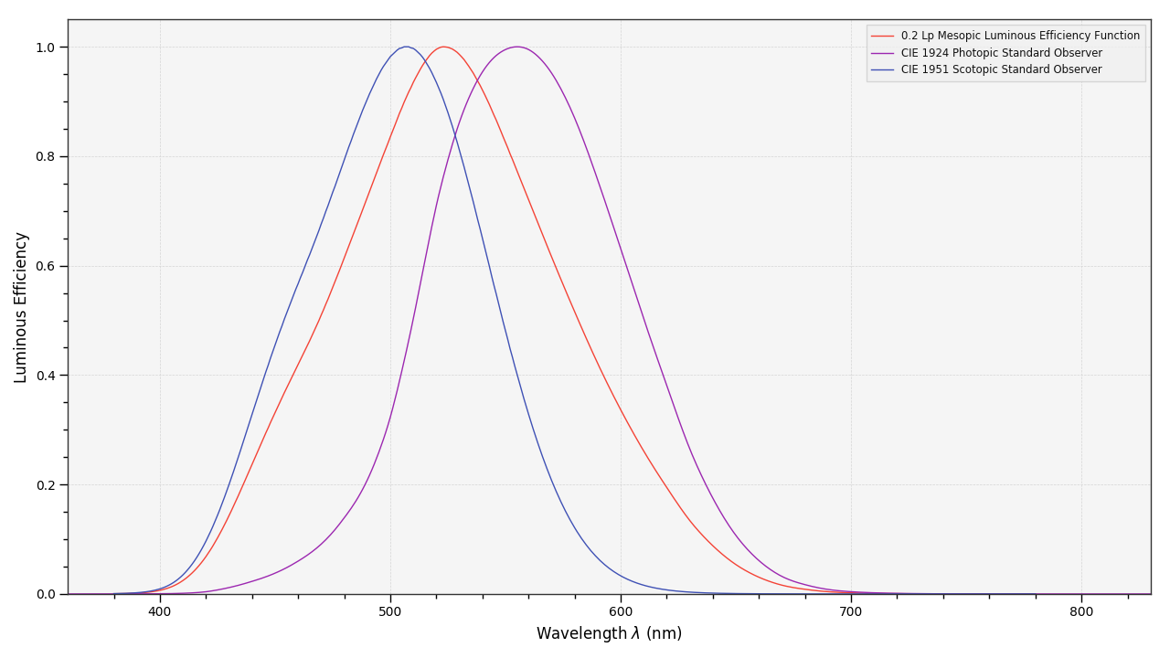
5.5.18.5 Luminous Efficiency
>>> sd_mesopic_luminous_efficiency_function = (
...     colour.sd_mesopic_luminous_efficiency_function(0.2))
>>> plot_multi_sds(
...     (sd_mesopic_luminous_efficiency_function,
...      colour.PHOTOPIC_LEFS['CIE 1924 Photopic Standard Observer'],
...      colour.SCOTOPIC_LEFS['CIE 1951 Scotopic Standard Observer']),
...     y_label='Luminous Efficiency',
...     legend_location='upper right',
...     y_tighten=True,
...     margins=(0, 0, 0, .1))
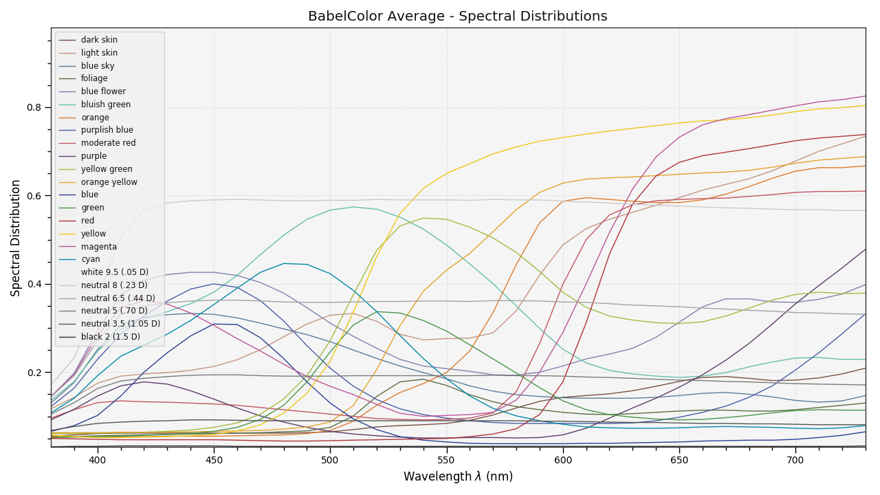
5.5.18.6 Colour Checker
>>> from colour.characterisation.dataset.colour_checkers.sds import (
...     COLOURCHECKER_INDEXES_TO_NAMES_MAPPING)
>>> plot_multi_sds(
...     [
...         colour.COLOURCHECKERS_SDS['BabelColor Average'][value]
...         for key, value in sorted(
...             COLOURCHECKER_INDEXES_TO_NAMES_MAPPING.items())
...     ],
...     use_sds_colours=True,
...     title=('BabelColor Average - '
...            'Spectral Distributions'))
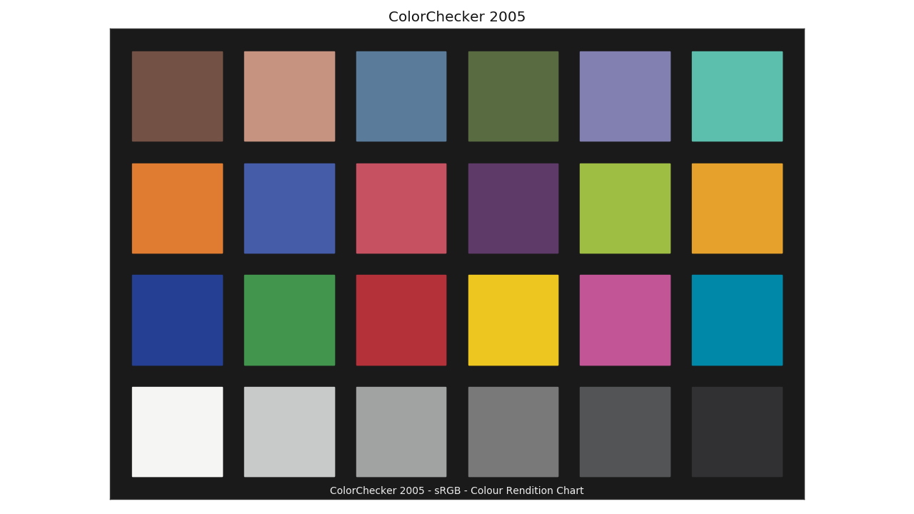
>>> plot_single_colour_checker('ColorChecker 2005', text_parameters={'visible': False})
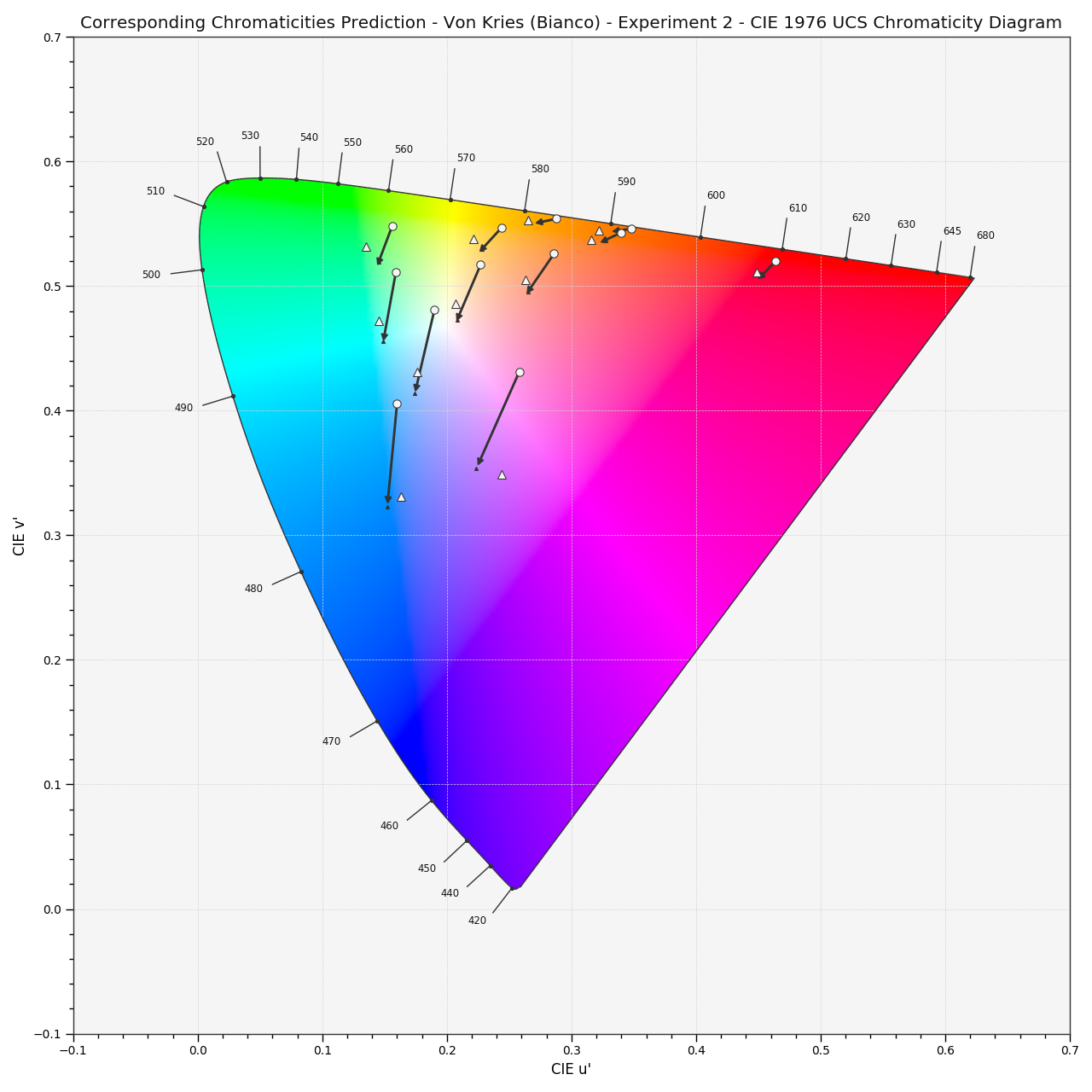
5.5.18.7 Chromaticities Prediction
>>> plot_corresponding_chromaticities_prediction(2, 'Von Kries', 'Bianco')
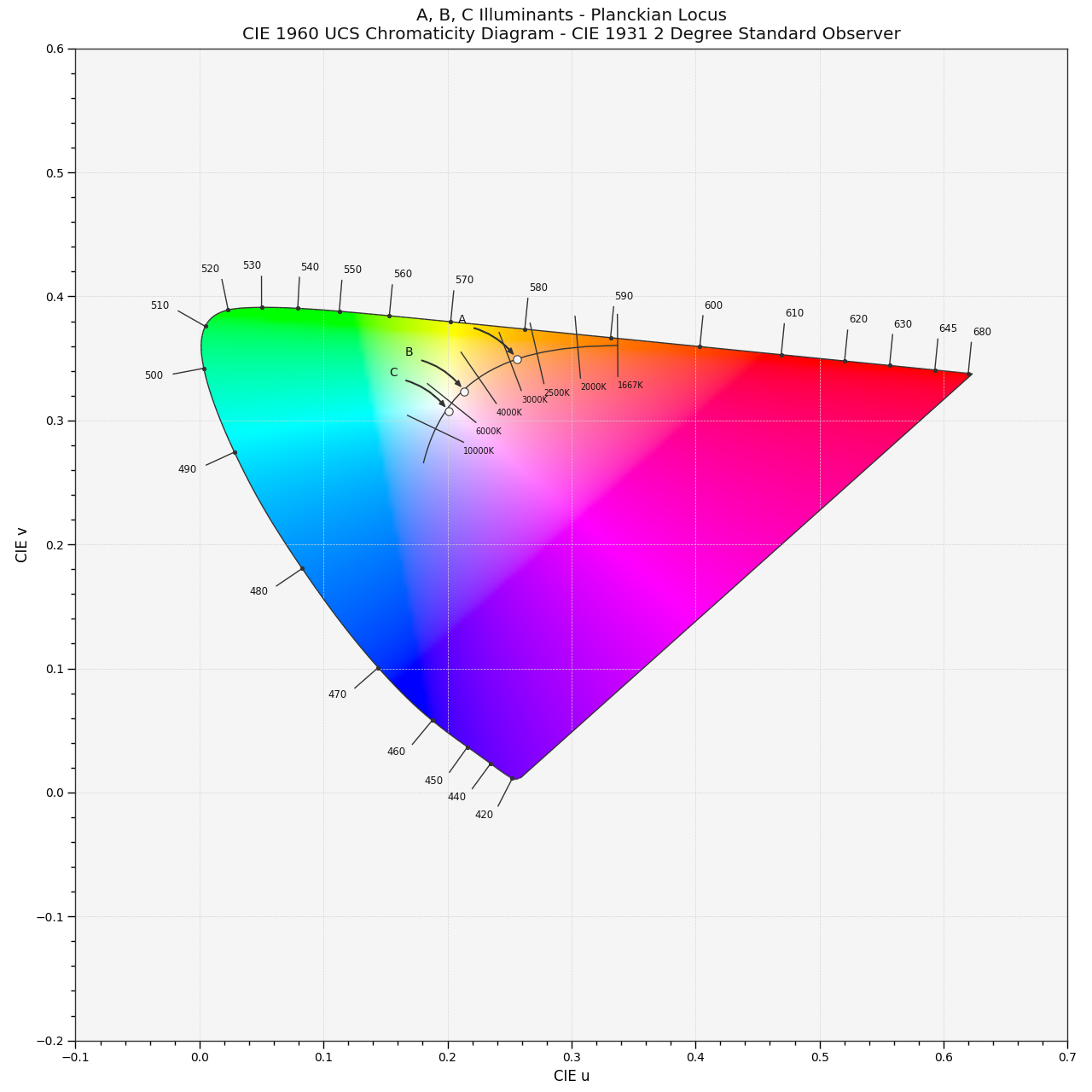
5.5.18.8 Colour Temperature
>>> plot_planckian_locus_in_chromaticity_diagram_CIE1960UCS(['A', 'B', 'C'])
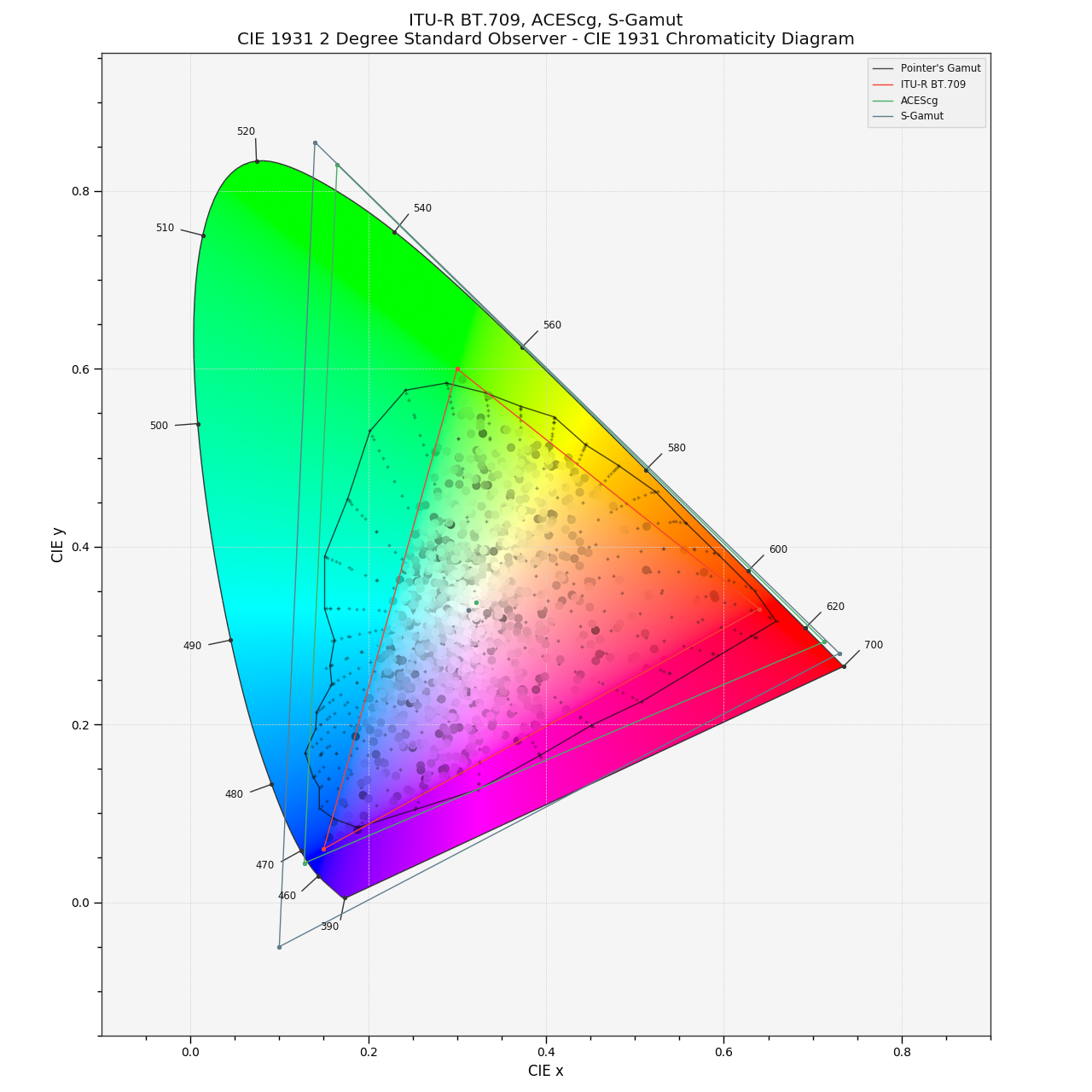
5.5.18.9 Chromaticities
>>> import numpy as np
>>> RGB = np.random.random((32, 32, 3))
>>> plot_RGB_chromaticities_in_chromaticity_diagram_CIE1931(
...     RGB, 'ITU-R BT.709', colourspaces=['ACEScg', 'S-Gamut'], show_pointer_gamut=True)
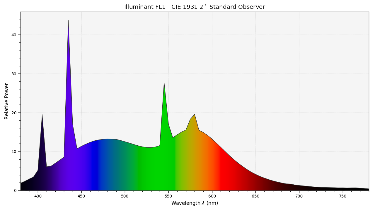
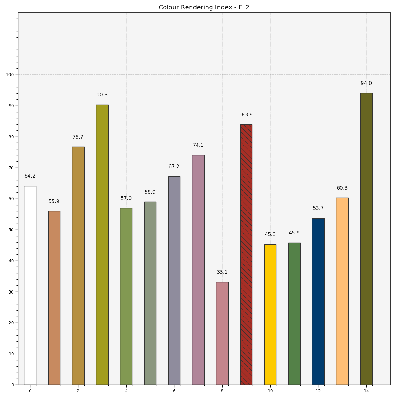
5.5.18.10 Colour Rendering Index
>>> plot_single_sd_colour_rendering_index_bars(
...     colour.ILLUMINANTS_SDS['FL2'])
6 Contributing
If you would like to contribute to Colour, please refer to the following Contributing guide.
8 Bibliography
The bibliography is available on the Bibliography page.
It is also viewable directly from the repository in BibTeX format.
9 See Also
Here is a list of notable colour science packages sorted by languages:
Python
Colorio by Schlömer, N.
ColorPy by Kness, M.
Colorspacious by Smith, N. J., et al.
python-colormath by Taylor, G., et al.
Go
go-colorful by Beyer, L., et al.
.NET
Colourful by Pažourek, T., et al.
Julia
Colors.jl by Holy, T., et al.
Matlab & Octave
COLORLAB by Malo, J., et al.
Psychtoolbox by Brainard, D., et al.
The Munsell and Kubelka-Munk Toolbox by Centore, P.
10 Code of Conduct
The Code of Conduct, adapted from the Contributor Covenant 1.4, is available on the Code of Conduct page.