colour.plotting.plot_constant_hue_loci¶

colour.plotting.plot_constant_hue_loci(data, model, scatter_kwargs=None, **kwargs)[source]¶

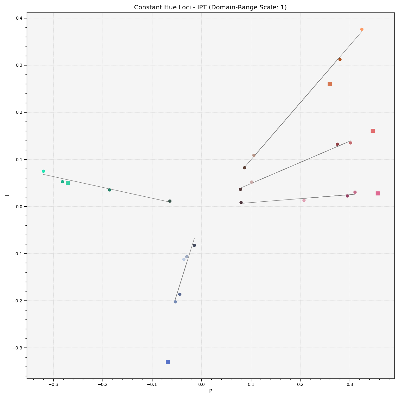
Plots given constant hue loci colour matches data such as that from [] or [] that are easily loaded with Colour - Datasets.

Parameters

data (array_like) –
Constant hue loci colour matches data expected to be an array_like as follows:
```
[
    ('name', XYZ_r, XYZ_cr, (XYZ_ct, XYZ_ct, XYZ_ct, ...), {metadata}),
    ('name', XYZ_r, XYZ_cr, (XYZ_ct, XYZ_ct, XYZ_ct, ...), {metadata}),
    ('name', XYZ_r, XYZ_cr, (XYZ_ct, XYZ_ct, XYZ_ct, ...), {metadata}),
    ...
]
```
where name is the hue angle or name, XYZ_r the CIE XYZ tristimulus values of the reference illuminant, XYZ_cr the CIE XYZ tristimulus values of the reference colour under the reference illuminant, XYZ_ct the CIE XYZ tristimulus values of the colour matches under the reference illuminant and metadata the dataset metadata.
model (unicode, optional) – {‘CIE XYZ’, ‘CIE xyY’, ‘CIE xy’, ‘CIE Lab’, ‘CIE LCHab’, ‘CIE Luv’, ‘CIE Luv uv’, ‘CIE LCHuv’, ‘CIE UCS’, ‘CIE UCS uv’, ‘CIE UVW’, ‘DIN 99’, ‘Hunter Lab’, ‘Hunter Rdab’, ‘IPT’, ‘JzAzBz’, ‘OSA UCS’, ‘hdr-CIELAB’, ‘hdr-IPT’}, Colourspace model.
scatter_kwargs (dict, optional) –
Keyword arguments for the plt.scatter() definition. The following special keyword arguments can also be used:
- c : unicode or array_like, if c is set to RGB, the scatter will use the colours as given by the RGB argument.
**kwargs (dict, optional) – {colour.plotting.artist(), colour.plotting.plot_multi_functions(), colour.plotting.render()}, Please refer to the documentation of the previously listed definitions. Also handles keywords arguments for deprecation management.

Returns

Current figure and axes.

Return type

tuple

References

[], [], []

Examples

>>> data = np.array([
...     [
...         None,
...         np.array([0.95010000, 1.00000000, 1.08810000]),
...         np.array([0.40920000, 0.28120000, 0.30600000]),
...         np.array([
...             [0.02495100, 0.01908600, 0.02032900],
...             [0.10944300, 0.06235900, 0.06788100],
...             [0.27186500, 0.18418700, 0.19565300],
...             [0.48898900, 0.40749400, 0.44854600],
...         ]),
...         None,
...     ],
...     [
...         None,
...         np.array([0.95010000, 1.00000000, 1.08810000]),
...         np.array([0.30760000, 0.48280000, 0.42770000]),
...         np.array([
...             [0.02108000, 0.02989100, 0.02790400],
...             [0.06194700, 0.11251000, 0.09334400],
...             [0.15255800, 0.28123300, 0.23234900],
...             [0.34157700, 0.56681300, 0.47035300],
...         ]),
...         None,
...     ],
...     [
...         None,
...         np.array([0.95010000, 1.00000000, 1.08810000]),
...         np.array([0.39530000, 0.28120000, 0.18450000]),
...         np.array([
...             [0.02436400, 0.01908600, 0.01468800],
...             [0.10331200, 0.06235900, 0.02854600],
...             [0.26311900, 0.18418700, 0.12109700],
...             [0.43158700, 0.40749400, 0.39008600],
...         ]),
...         None,
...     ],
...     [
...         None,
...         np.array([0.95010000, 1.00000000, 1.08810000]),
...         np.array([0.20510000, 0.18420000, 0.57130000]),
...         np.array([
...             [0.03039800, 0.02989100, 0.06123300],
...             [0.08870000, 0.08498400, 0.21843500],
...             [0.18405800, 0.18418700, 0.40111400],
...             [0.32550100, 0.34047200, 0.50296900],
...             [0.53826100, 0.56681300, 0.80010400],
...         ]),
...         None,
...     ],
...     [
...         None,
...         np.array([0.95010000, 1.00000000, 1.08810000]),
...         np.array([0.35770000, 0.28120000, 0.11250000]),
...         np.array([
...             [0.03678100, 0.02989100, 0.01481100],
...             [0.17127700, 0.11251000, 0.01229900],
...             [0.30080900, 0.28123300, 0.21229800],
...             [0.52976000, 0.40749400, 0.11720000],
...         ]),
...         None,
...     ],
... ])
>>> plot_constant_hue_loci(data, 'IPT')  
(<Figure size ... with 1 Axes>, <...AxesSubplot...>)