colour.plotting.temperature.plot_planckian_locus#
- colour.plotting.temperature.plot_planckian_locus(planckian_locus_colours: ArrayLike | str | None = None, planckian_locus_opacity: float = 1, planckian_locus_labels: Sequence | None = None, planckian_locus_mireds: bool = False, planckian_locus_iso_temperature_lines_D_uv: float = 0.05, method: Literal['CIE 1931', 'CIE 1960 UCS', 'CIE 1976 UCS'] | str = 'CIE 1931', **kwargs: Any) Tuple[Figure, Axes][source]#
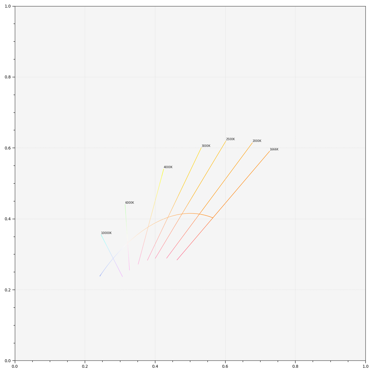
Plot the Planckian Locus using the specified method.
- Parameters:
planckian_locus_colours (ArrayLike | str | None) – Colours of the Planckian Locus, if
planckian_locus_coloursis set to RGB, the colours will be computed using the corresponding chromaticity coordinates.planckian_locus_opacity (float) – Opacity of the Planckian Locus.
planckian_locus_labels (Sequence | None) – Array of labels used to customise which iso-temperature lines will be drawn along the Planckian Locus. Passing an empty array will result in no iso-temperature lines being drawn.
planckian_locus_mireds (bool) – Whether to use micro reciprocal degrees for the iso-temperature lines.
planckian_locus_iso_temperature_lines_D_uv (float) – Iso-temperature lines \(\Delta_{uv}\) length on each side of the Planckian Locus.
method (Literal['CIE 1931', 'CIE 1960 UCS', 'CIE 1976 UCS'] | str) – Chromaticity Diagram method.
kwargs (Any) – {
colour.plotting.artist(),colour.plotting.render()}, See the documentation of the previously listed definitions.
- Returns:
Current figure and axes.
- Return type:
Examples
>>> plot_planckian_locus(planckian_locus_colours="RGB")
...
(<Figure size ... with 1 Axes>, <...Axes...>)