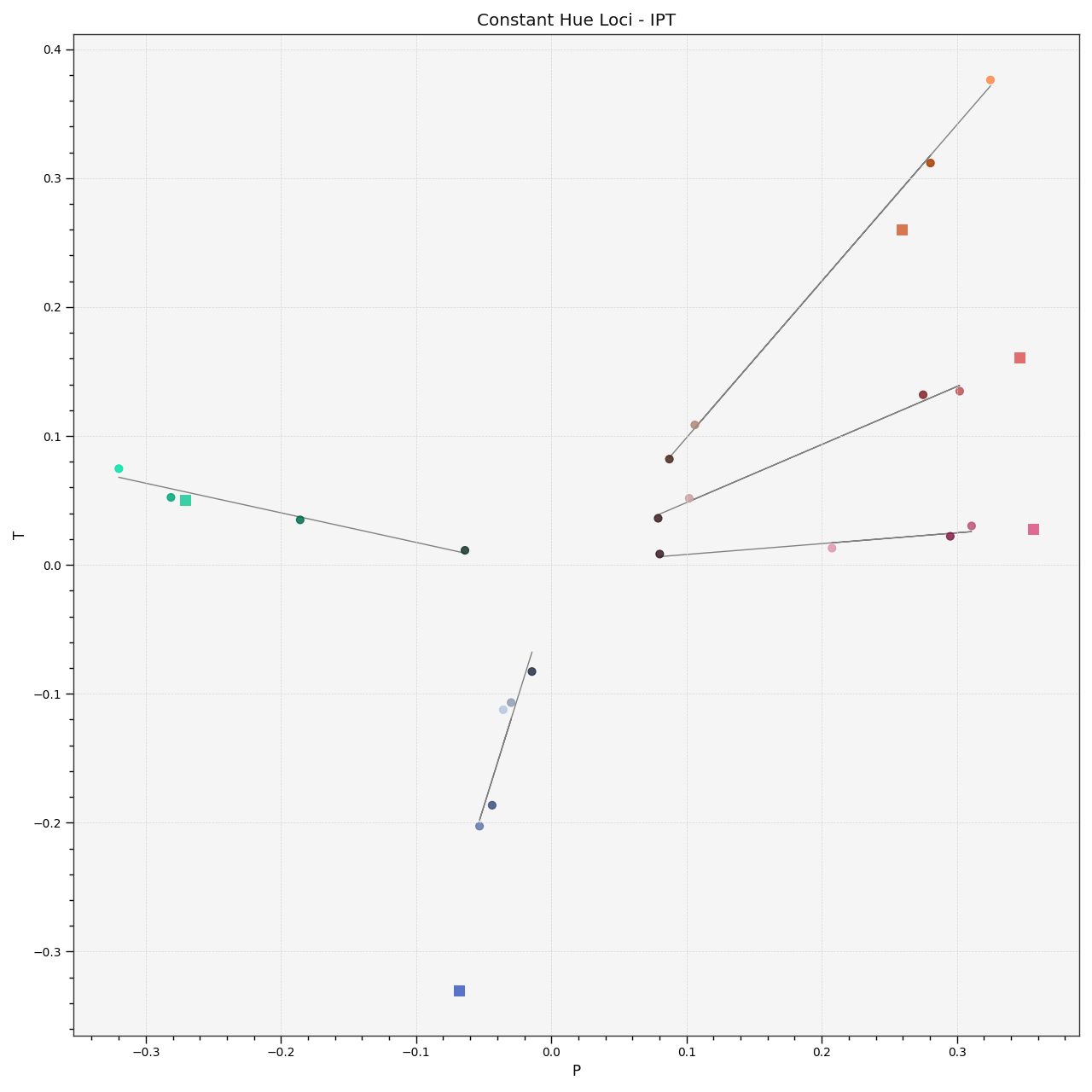
colour.plotting.plot_constant_hue_loci#

colour.plotting.plot_constant_hue_loci(data: ArrayLike, model: LiteralColourspaceModel | str = 'CIE Lab', scatter_kwargs: dict | None = None, convert_kwargs: dict | None = None, **kwargs: Any) → Tuple[Figure, Axes][source]#

Plot given constant hue loci colour matches data such as that from [HB95] or [EF98] that are easily loaded with Colour - Datasets.

Parameters:

data (ArrayLike) –
Constant hue loci colour matches data expected to be an ArrayLike as follows:
```
[
    ('name', XYZ_r, XYZ_cr, (XYZ_ct, XYZ_ct, XYZ_ct, ...),     {metadata}),
    ('name', XYZ_r, XYZ_cr, (XYZ_ct, XYZ_ct, XYZ_ct, ...),     {metadata}),
    ('name', XYZ_r, XYZ_cr, (XYZ_ct, XYZ_ct, XYZ_ct, ...),     {metadata}),
    ...
]
```
where name is the hue angle or name, XYZ_r the CIE XYZ tristimulus values of the reference illuminant, XYZ_cr the CIE XYZ tristimulus values of the reference colour under the reference illuminant, XYZ_ct the CIE XYZ tristimulus values of the colour matches under the reference illuminant and metadata the dataset metadata.
model (LiteralColourspaceModel | str) – Colourspace model, see colour.COLOURSPACE_MODELS attribute for the list of supported colourspace models.
scatter_kwargs (dict | None) –
Keyword arguments for the matplotlib.pyplot.scatter() definition. The following special keyword arguments can also be used:
- c : If c is set to RGB, the scatter will use the colours as given by the RGB argument.
convert_kwargs (dict | None) – Keyword arguments for the colour.convert() definition.
kwargs (Any) – {colour.plotting.artist(), colour.plotting.plot_multi_functions(), colour.plotting.render()}, See the documentation of the previously listed definitions.

Returns:

Current figure and axes.

Return type:

tuple

References

[EF98], [HB95], [Man19]

Examples

>>> data = [
...     [
...         None,
...         np.array([0.95010000, 1.00000000, 1.08810000]),
...         np.array([0.40920000, 0.28120000, 0.30600000]),
...         np.array(
...             [
...                 [0.02495100, 0.01908600, 0.02032900],
...                 [0.10944300, 0.06235900, 0.06788100],
...                 [0.27186500, 0.18418700, 0.19565300],
...                 [0.48898900, 0.40749400, 0.44854600],
...             ]
...         ),
...         None,
...     ],
...     [
...         None,
...         np.array([0.95010000, 1.00000000, 1.08810000]),
...         np.array([0.30760000, 0.48280000, 0.42770000]),
...         np.array(
...             [
...                 [0.02108000, 0.02989100, 0.02790400],
...                 [0.06194700, 0.11251000, 0.09334400],
...                 [0.15255800, 0.28123300, 0.23234900],
...                 [0.34157700, 0.56681300, 0.47035300],
...             ]
...         ),
...         None,
...     ],
...     [
...         None,
...         np.array([0.95010000, 1.00000000, 1.08810000]),
...         np.array([0.39530000, 0.28120000, 0.18450000]),
...         np.array(
...             [
...                 [0.02436400, 0.01908600, 0.01468800],
...                 [0.10331200, 0.06235900, 0.02854600],
...                 [0.26311900, 0.18418700, 0.12109700],
...                 [0.43158700, 0.40749400, 0.39008600],
...             ]
...         ),
...         None,
...     ],
...     [
...         None,
...         np.array([0.95010000, 1.00000000, 1.08810000]),
...         np.array([0.20510000, 0.18420000, 0.57130000]),
...         np.array(
...             [
...                 [0.03039800, 0.02989100, 0.06123300],
...                 [0.08870000, 0.08498400, 0.21843500],
...                 [0.18405800, 0.18418700, 0.40111400],
...                 [0.32550100, 0.34047200, 0.50296900],
...                 [0.53826100, 0.56681300, 0.80010400],
...             ]
...         ),
...         None,
...     ],
...     [
...         None,
...         np.array([0.95010000, 1.00000000, 1.08810000]),
...         np.array([0.35770000, 0.28120000, 0.11250000]),
...         np.array(
...             [
...                 [0.03678100, 0.02989100, 0.01481100],
...                 [0.17127700, 0.11251000, 0.01229900],
...                 [0.30080900, 0.28123300, 0.21229800],
...                 [0.52976000, 0.40749400, 0.11720000],
...             ]
...         ),
...         None,
...     ],
... ]
>>> plot_constant_hue_loci(data, "CIE Lab")  
(<Figure size ... with 1 Axes>, <...Axes...>)

colour.plotting.plot_constant_hue_loci#

This Page