colour.plotting.diagrams.plot_chromaticity_diagram_colours
- colour.plotting.diagrams.plot_chromaticity_diagram_colours(samples: Integer = 256, diagram_colours: Optional[Union[ArrayLike, str]] = None, diagram_opacity: Floating = 1, diagram_clipping_path: Optional[ArrayLike] = None, cmfs: Union[MultiSpectralDistributions, str, Sequence[Union[MultiSpectralDistributions, str]]] = 'CIE 1931 2 Degree Standard Observer', method: Union[Literal['CIE 1931', 'CIE 1960 UCS', 'CIE 1976 UCS'], str] = 'CIE 1931', **kwargs: Any) Tuple[plt.Figure, plt.Axes][source]
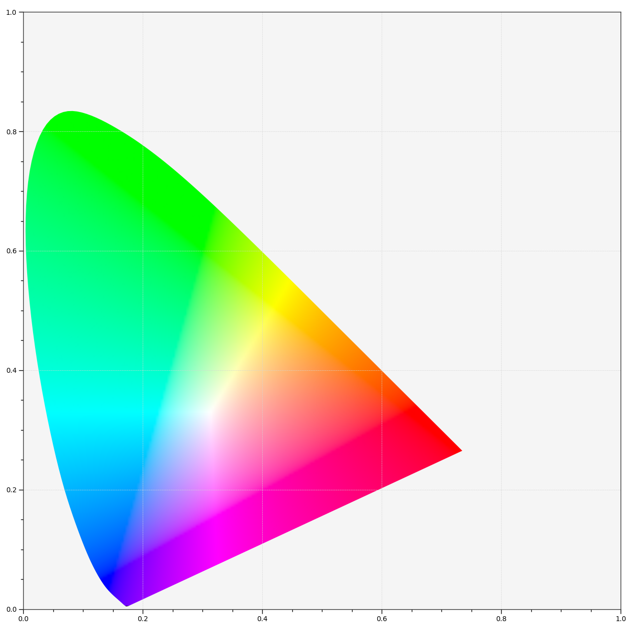
Plot the Chromaticity Diagram colours according to given method.
- Parameters
samples (Integer) – Samples count on one axis when computing the Chromaticity Diagram colours.
diagram_colours (Optional[Union[ArrayLike, str]]) – Colours of the Chromaticity Diagram, if
diagram_coloursis set to RGB, the colours will be computed according to the corresponding coordinates.diagram_opacity (Floating) – Opacity of the Chromaticity Diagram.
diagram_clipping_path (Optional[ArrayLike]) – Path of points used to clip the Chromaticity Diagram colours.
cmfs (Union[MultiSpectralDistributions, str, Sequence[Union[MultiSpectralDistributions, str]]]) – Standard observer colour matching functions used for computing the spectral locus boundaries.
cmfscan be of any type or form supported by thecolour.plotting.filter_cmfs()definition.method (Union[Literal[('CIE 1931', 'CIE 1960 UCS', 'CIE 1976 UCS')], str]) – Chromaticity Diagram method.
kwargs (Any) – {
colour.plotting.artist(),colour.plotting.render()}, See the documentation of the previously listed definitions.
- Returns
Current figure and axes.
- Return type
Examples
>>> plot_chromaticity_diagram_colours(diagram_colours='RGB')
...
(<Figure size ... with 1 Axes>, <...AxesSubplot...>)